 Richard Llewellyn Langford
- Consultant, Viana do Castelo, Portugal
The Granites-Tanami Orogen (GTO) is a significant auriferous province located in the poorly exposed southwestern part of the North Australian Craton. This paper looks at the data sources that are suited to studying regolith-landform in areas such as the Tanami Region. One of the most useful datasets for regional regolith-landform mapping is a digital elevation model (DEM). The DEM data that were reviewed demonstrated the utility of TanDEM over other sources, and quantitative results focused on these data for identifying regolith-landform patterns that would aid in geochemical sampling and other land use studies. This paper will demonstrate that neither the classical approach of mapping boundaries based on visual estimates of breaks in slope, nor the alternative approach of producing maps and models derived from algorithms, can be used in isolation. Visual estimates of many boundaries are complex, unreliable and time consuming, and algorithmic mapping is driven by parameters than can produce an infinite set of models. This paper shows that simple landform visualisation is often the most powerful tool for map and model creation, supported by geomorphometric analysis and remotely sensed spectral imagery. The use of TanDEM data is shown to produce the best regolith-landform maps and models of the Tanami Region, which can then improve mineral exploration success.
Introduction
This paper covers the Tanami Region (Bain and Draper, 1998; Blake and Kilgour, 1998; Pain, 2008) and adjacent parts of the Birrindudu Region to the west, the Wiso Region to the northeast and the Arunta Region to the southeast (Figure 1). The interpretation also extends west of the Birrindudu Region into the margin of the Canning Basin. The Tanami Region is a poorly exposed, mostly Paleoproterozoic province within Northern Australia that hosts a number of significant gold deposits (Plumb et al., 1990; Smith et al., 1998; Huston et al., 2007; Bagas et al., 2009). The Callie deposit is the largest (6.0 Moz Au) and is hosted by black mudstones of the Dead Bullock Formation (Smith et al., 1998). Effective mineral exploration of the Tanami has been severely hampered by poor knowledge of the regional stratigraphy, as it is difficult to identify and correlate exposed packages of poorly-sorted sandstones, siltstones and black mudstones separated by large regions of regolith cover (Blake et al., 1979; Hendrickx et al., 2000; Crispe et al., 2007; Huston et al., 2007).

Figure 1. Location of the Tanami Region, Australia (yellow) and project area (red); GDA94.
Transported regolith thicknesses in the Tanami vary from quite minor (sub-cropping bedrock) to over 100 m within palaeochannel systems (Reid et al., 2005). These palaeochannels are important in mineral exploration (Jiang et al., 2019), as they may contain remobilised gold, uranium, and heavy minerals (Hou et al., 2008), and in groundwater exploration, as they often form productive aquifers (Mulligan et al., 2007; Samadder et al., 2011; Knight et al., 2018). For example, valley fills and palaeochannel sediments may contain alluvial gold that can be traced back to original source areas (Gozzard, 2004), although exploration for mineral deposits can be complicated in areas where the palaeodrainage is covered by alluvial fans that partially bury former basement topography defined by palaeovalleys and ridges (Mote et al., 2001). Many palaeovalleys originated as Permian glacial valleys, particularly in upland areas of Archean to Proterozoic bedrock (English et al., 2012).
The most common expression of a significant change in the nature of geological materials at the surface of the Earth, the regolith, is a change in the landform or terrain. Observing variations in landform using regolith-landform maps is at the core of classical geological mapping, and is the mainstay of many mapping agencies. As a result, our understanding of the intimate relationship between landform, material, and process at the surface is constantly improving. Understanding change in the landscape has always been a key part of geological mapping, and is fundamental to the creation of regolith-landform maps that can improve mineral exploration success. A regolith-landform map will primarily be a map of changes or breaks in slope that defines landform patterns or elements, and is combined with the material composition, and an understanding of active and relict processes, to produce a complete map.
This paper is focused on the best digital elevation model (DEM) data to use in areas of very low relief, and examines the benefits of using TanDEM-X radar interferometry-derived elevation data (Moreira et al., 2004; Krieger et al., 2007) in the Tanami Region of northern Australia, a highly prospective and very poorly exposed terrain (Figure 1). The Tanami was chosen for study not only because of its prospectivity, but also because previous work had struggled to produce a coherent picture of the regolith-landforms in the very low relief that dominates the area. Figure 2 shows that there is clearly a complex landform pattern at a regional-scale that would justify more detailed analysis.
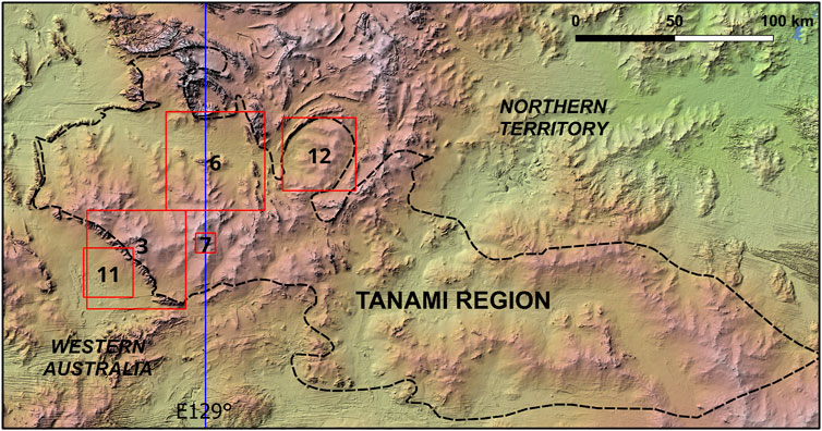
Figure 2. Project Area elevation (235–715 m AHD) with northwest illumination; Tanami Region (black dash); locations and number of figures (red), and WA-NT border (blue).
The past few decades have seen increased use made of remotely sensed data and image products by geoscientists to improve regolith-landform mapping. Datasets used routinely include DEMs, Landsat Thematic Mapper (TM), and airborne gamma ray spectrometry (radiometrics). Remotely sensed data, however, typically lack the essential landform context provided by three-dimensional control. Only recently have widely available advances been made in bringing together the power of both remotely sensed imagery and detailed landform models using DEMs. This paper is focused on the use of DEMs to produce a model that can be integrated with other data sources such as remotely sensed imagery, radiometrics and pre-existing geological interpretations. Landform elements and landform patterns are described and classified into named types by the values of their landform attributes (Speight, 2009).
Regolith-landform maps provide an important geomorphological and landscape evolution framework for developing effective geochemical exploration strategies (Wilford and Butrovski, 2000), and in the interpretation of geochemical datasets in subdued terrains such as the Tanami. Identifying pathways of geochemical dispersion in the landscape relies on mapping both the bedrock geology and the regolith, and the development of regolith-landform maps is an attempt to represent multiple perspectives of three-dimensional surfaces in a two-dimensional image.
Although landforms undoubtedly reflect changes and variations in lithological characteristics and geological structures, a common error among geologists is that they regard landforms solely as a result of the geological setting. The age of a feature, length of time one or more processes have been operating, and the sequence of events all play a role in the evolution of a landscape (Gozzard and Langford, 2004).
Information and Data Sources
The sources of information and data used in regolith-landform mapping in the Tanami include both classification systems and the types of data that can be used in this new mapping. The most useful types of data for regional regolith-landform mapping, in addition to a good understanding of the underlying geology and mineralisation, are primarily DEMs, and both multispectral and radiometric imagery. Research and map development for the Tanami has therefore focused on improving the spatial analysis of DEMs, with limited input from Landsat TM, the coarser radiometric data and high resolution satellite imagery.
Landform Classification
The Tanami can be classified using simple types of erosional and aggradational landform pattern characterised by relief and modal slope (Table 5 in Speight, 2009). The most rugged parts of the landscape have a relief of around 100 m, and this is mostly in the hills and scarps on the edge of the Tanami, and not within it. Most of the relief within the Tanami is around 50 m, giving an overall relief ranking of low (L; 30–90 m; ∼50 m). However, most of the slopes are level (LE; <1%), so have no classification in Speight’s table. There is no classification system in use in Australia that distinguishes large-scale, low relief landforms from level plains, despite the appearance of the landscape being dominated by low hills with intervening broad valleys. The conventional definition of a low hill is that it should have slopes of 10%–32% (Table 7 in Speight, 2009).
Landform Mapping
Mapping regolith in Australia is largely based on the approach defined by Christian et al. (1953), who defined a new unit, the Land System, as a composite of related units, as an area, or groups of areas, throughout which there is a recurring pattern of topography, soils, and vegetation. They also noted that geomorphological processes are more important than the basic geological material, although the two are obviously related.
The national system used by Geoscience Australia, RTMAP (Pain et al., 2000; Pain et al., 2007), has regolith type closely associated with landforms and with geomorphic processes. This uses landforms as a surrogate for regolith (Chan, 1988), with origins in techniques developed for mapping landforms and soil (Stewart and Perry, 1953; Ollier, 1977). Geoscience Australia and CRC LEME map Regolith Landform Units (RLU; Chan, 1988) comprise one or more recurring landscape elements and their associated underlying regolith packages. Although the mapping system used to create RLUs is complex, with a focus on field observation, a primary principle is the identification of landforms. A derivative approach (Hocking et al., 2007) used in Western Australia uses landform and process as the dominant classification characteristic, with a range of other qualifiers dealing with relative age and material.
Effective regolith-landform mapping relies on identifying the morphology, process and material of any mappable area or unit. The Australian landform classification system (Eggleton, 2000; Speight, 2009) has been used to define all the features that can be identified and mapped in the region.
Digital Elevation Models
Only recently has the production of freely available DEMs of large areas with acceptable horizontal and vertical resolution been commonplace with the introduction of a number of satellite based systems, notably the Shuttle Radar Topography Mission (SRTM; Earth Resources Observation And Science (EROS) Center, 2017a), the Advanced Spaceborne Thermal Emission and Reflection Radiometer (ASTER) Global Digital Elevation Model (GDEM), the Advanced Land Observing Satellite “Daichi” (ALOS) and TanDEM-X (TanDEM; Moreira et al., 2004; Krieger et al., 2007). Prior to the use of satellite data, DEMs could be created using digitised land survey data, such as spot heights, contours and base station points, or using stereo aerial photography with ground control.
The GEODATA 9 Second DEM (DEM-9S) is a grid of ground level elevation points covering the whole of Australia, with a grid spacing of 9 arcseconds in longitude and latitude (approximately 250 m) in the GDA94 coordinate system. Version 1 of the 9 Second DEM (Carroll and Morse, 1996) was used by Wilford and Butrovski (1999), and the latest version (Version 3; Geoscience Australia et al., 2008) was used in this paper solely for comparative purposes (Figure 3A). Despite the softness of the images resulting from the wide grid spacing, the DEM-9S provides better insights into the variety of landforms than some of the higher resolution datasets such as SRTM1 and ASTER.
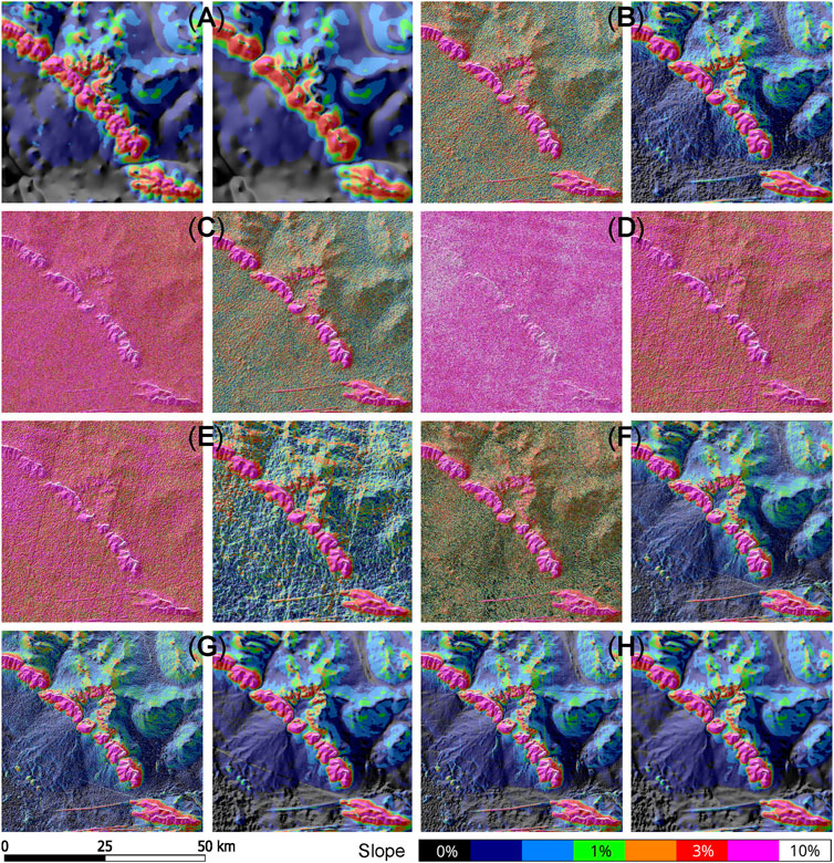
Figure 3. Review of image pairs of slope classes for raw data and 21 × 21 multi-scale resampled data (Wood, 1996; Wood, 2009) with aspect bias northwest illumination: (A) GEODATA DEM-9S (250 m), (B) SRTM3 (90 m), (C) SRTM1 (30 m), (D) ASTER (30 m), (E) ASTER resampled (90 m), (F) ALOS (30 m), (G) ALOS resampled (90 m) and (H) TanDEM (90 m); centred on MGA Zone 52 K 465000E 7765000N, 72 km east of Balgo Community, Western Australia. Level (LE <1%), very gently inclined (VG 1%–3%), gently inclined (GE 3%–10%), and steeper slope over 10%.
SRTM 3 arcseconds global coverage (SRTM3, ∼90 m) is freely available to the public, and these data were used in preliminary mapping of the Tanami in Western Australia (Figure 3B; Langford, 2007). In late 2014, the release of the 30-m resolution SRTM1 DEM did not yield a useful improvement in areas such as the Tanami (Figure 3C; Earth Resources Observation And Science (EROS) Center, 2017b). Although the data are not necessarily representative of the ground surface, but the top of whatever is first encountered by the radar, this is not an issue in desert areas such as the Tanami that have no tall vegetation. There is, however, an issue with the precision of the data, for which elevation values are supplied as integers. In areas of very low topography this makes slope calculations very difficult to interpret. Multi-scale resampling of the elevation can be used to generate a set of real numbers for elevation that go some way to correcting this problem (Figure 3; Langford, 2007).
ASTER GDEM is a notionally much higher quality 30-m resolution DEM than SRTM that is also freely available for 99% of the globe. ASTER GDEM used stereoscopic pairs and digital image correlation methods. Version 3 is claimed to have significant improvements over the previous release and is used in this paper (Figures 3D, E). Despite being considered a more accurate representation than the SRTM elevation model in rugged mountainous terrain, this paper will demonstrate that in areas of very low relief with sparse vegetation there are issues with the utility of stereoscopically acquired data, both because the methodology is not well suited to that terrain and because the precision of the data has elevation values supplied as integers, not real numbers.
ALOS data are supplied at a global 1 arcsecond resolution (30 m). As with both SRTM and ASTER data the precision of the data has elevation values supplied as integers, not real numbers, and like ASTER the utility of stereoscopically acquired data is not well suited to that terrain with very low relief and few surface features (Figures 3F, G).
TanDEM uses the TerraSAR-X SAR interferometer built by two almost identical satellites flying in close formation (Moreira et al., 2004; Krieger et al., 2007). The TanDEM 90 m DEM is derived from the global DEM with a 0.4 arcseconds (12 m) posting, and has a reduced pixel spacing of 3 arcseconds (Figure 3H), with a vertical accuracy of 2 m (relative) and 4 m (absolute).
Review of Different DEM Datasets
The capacity for any DEM to provide useful landform imagery, or to be a suitable source for geomorphometric analysis, needs to be tested before embarking on more detailed analysis. The six DEM sources reviewed are GEODATA 9 s DEM (DEM-9S), ASTER, SRTM3, SRTM1, ALOS and TanDEM. All are derived from satellite observations except the DEM-9S, which was compiled from historical ground observations and photogrammetry, and is included because it was the primary landform source used by Wilford and Butrovski (1999). An earlier study of landform in the Tanami was completed using SRTM3 data and multi-scale resampling in LandSerf (Wood, 1996; Langford, 2007; Wood, 2009; Langford, 2015). This earlier work showed that it was possible to significantly improve visualisation of SRTM3 data, allowing hitherto invisible or obscure landforms to be identified. The multi-scale sampling window size of 21 × 21 pixels was chosen based simply on the preferred visualisation.
The comparison of images in Figures 3A–H shows that multi-scale resampling cannot improve the oldest DEM-9S (Figure 3A) or produce useful images for SRTM1 (Figure 3C) or ASTER (Figure 3D), even when resampled to 90 m (Figure 3E). Multi-scale resampling was needed to produce useful images for SRTM3 (Figure 3B) and ALOS (Figure 3F), although ALOS data are also easier to process if resampled to 90 m (Figure 3G). The TanDEM (Figure 3H) dataset is the only one that can be used with confidence in its raw form or resampled, and this can be attributed to two factors. The first is the poor performance of DEMs created using stereo pairs in areas of very low relief with few distinguishing ground features (DEM-9S, ASTER and ALOS), and second is the non-integer nature of all the data except DEM-9S and TanDEM, which in areas of very low relief creates a stepped or banded appearance.
Slope Classification
Key to understanding landforms in areas of very low relief is an appreciation of variations in slope. The slope is typically also an integral part of the assignation to a specific landform pattern or element (Speight, 2009; Dobos et al., 2010), with the Australian system used for this paper (Table 1). A simple northwest illuminated shaded relief image using TanDEM data (Figure 2) gives the impression that there is a complex set of landforms, with ridges, hills, fans and valleys all visible. The landform classification system (Speight, 2009) assumes that most of these landforms would have a gently or very gently inclined slope, which means greater than 1%. Landforms less than 1% are typically designated as plains or plateaus, but the Tanami is dominated by slopes of less than 1%.
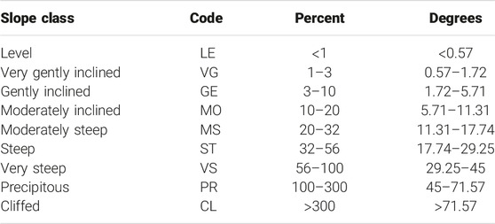
Table 1. Definition of slope class boundaries (After Speight, 2009).
Only when slopes both less than 0.2% and less than 0.4% are highlighted (Figure 4) are the landforms that are clearly visible in the simple shaded relief image now partially defined, with major drainage channels clearly separated and some definition in fans and other slope related features. This simple slope classification provides only an indication of the potential complexity of the landform patterns, and this paper is designed to elucidate those patterns.
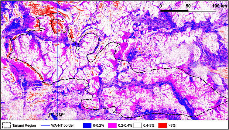
Figure 4. Tanami Region (black dash) with areas underlain by level to very gently inclined slopes <0.2% (red), <0.4% (green), and white (0.4%–3%), and gently inclined to steep slopes >3% (blue).
Landsat TM
One of the most useful additional datasets for regional regolith-landform mapping is spectral imagery such as Landsat TM. Landsat TM has been a mainstay for geologists for many years, and contains information on landscape pattern and temporal changes that are potentially underutilised in regolith-landform and bedrock mapping. Combining spectral data from Landsat TM with landform models provides an opportunity to create more detailed maps prior to commencing field activities, particularly when mapping the regolith. Experience has shown (Gozzard and Tapley, 1994; Tapley and Gozzard, 1994) that two image enhancements in particular are able to effectively discriminate and identify a wide range of geological and regolith materials, namely, interband ratios of bands 5/7:4/7:4/2, and a decorrelation stretch image of bands 4:5:7 (RGB; Figure 5). Using temporal merging the resulting images have fewer short-term responses such as fire scars and floods (Langford, 2015).
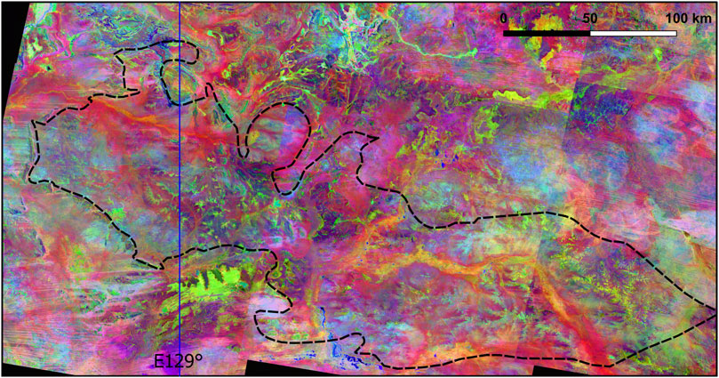
Figure 5. Decorrelation stretch image of bands 4:5:7 (RGB) for temporally merged Landsat TM 1990–2013 (Langford, 2015); Tanami Region (black dash).
Radiometrics
Airborne gamma-ray spectrometry (radiometrics) is an effective mapping tool in many different environments (Wilford, 1995; Gozzard, 2004), and has been used mainly as a tool for lithological mapping and in mineral exploration. Across the Tanami, KTU RGB radiometric images have been incorporated in geological maps of The Granites (Slater, 2000b; Vandenburg and Crispe, 2014), Mount Solitaire (Crispe et al., 2005), and Tanami (Slater, 2000a; Hendrickx et al., 2000) and posters (GSWA, 2009; de Souza Kovacs, 2013), although specific discussion of the use of airborne radiometrics to distinguish lithologies is found only in Hendrickx et al. (2000).
Interpretation Methodology
There are two broad approaches used in this paper to compiling a regolith-landform map suitable for predictive geological mapping and geochemical sampling. The classical approach is visualising a landscape using imagery derived from elevation data and then mapping boundaries based on visual estimates of breaks in slope, as they are the defining characteristic for most mappable changes. The second approach that was used is to produce maps and models derived from algorithms designed to characterise the landscape. In both cases, the mapping is usually combined with other imagery, such as Landsat and radiometrics, that reinforces or characterises differences mapped on the basis of landform. This paper will demonstrate that currently neither approach can be used in isolation, as visual estimates of boundaries are complex, unreliable and time consuming, and algorithmic mapping is driven by parameters than can potentially produce an infinite set of models. A combination of processing the DEM data and visualisation of the result is proposed as the best method for producing a regolith-landform map, although future trends in processing may reduce the need for manual intervention (Diaby et al., 2023).
Landform, Process and Material
Creating a regolith-landform map is achieved by understanding and either mapping or modelling three components; landform, process and material. Understanding each of these components is not always straightforward, especially in terrains such as those found in Australia that have a very long and varied regolith history (Ollier, 1977; Gozzard, 2004; Bourne and Twidale, 2010). As a landform is simply a shape in the landscape, of a particular scale and complexity, this is usually the easiest component to study at a regional-scale. The process that created the landform may not be the process or processes currently active, so any interpretation of process has to be presented in a way that makes sense in a landform context, but does not ignore the impact of landform modifying processes. The third component, material, is both the hardest to predict and the most complex (Gozzard, 2004; Hocking et al., 2007). Spectral or field observation of the landform surface will often be an unreliable determinant of the composition of the landform in 3-D. This means that the landform, the processes creating or acting on a landform, and the composition of the landform must be treated separately. Of the three, only the landform, which is an observable 3-D form, is an absolute, whereas process and material will be variables that lie within or across landforms, and may or may not be linked to the creation of the landform.
Data Processing and Visualisation
Keys to understanding landform elements and patterns are relief, slope and morphology (Speight, 2009), with morphology determined by a combination of curvature and position in the landscape. A change in curvature can be a sharp break, for example, on a cliff or escarpment, or a more subtle change, for example, from a hill crest to a hill slope. Regardless, the visualisation of a change in slope can be used to define or subdivide a landform, and is key to creating a regolith-landform map. The single most important aspect of the terrain to identify is a downslope break in slope, which in the Tanami is a slope change of as little as 0.2%.
Multi-Scale Resampling
The raw 90-m data resolution TanDEM data do not always yield the most useful results, both in terms of data processing and image complexity. The raw data contains artefacts and noise that especially impacts in areas of very low relief. Using LandSerf multi-scale resampling (Wood, 1996) of the elevation before extracting geomorphometric data and images is an ideal way of improving landform visualisation without losing all the detail that simple smoothing would do. For this paper a variety of window scales have been trialled, and the data were multi-scale resampled with a 21 × 21 window with a varying exponent that reduced extraneous detail to differing degrees.
Relief, Contours and Slope
Following the classical or conventional mapping technique, the first approach to mapping boundaries in this paper is to use the basic topographic elements of relief, contour inflections and slope images. Using these data and images allows clear breaks in slope or recognisable landforms to be delineated. There are several approaches in the use of shaded relief images; one is to use conventional vertical exaggeration, and another is to use aspect shading (Wood, 1996). In addition, this can be applied to raw data or multi-scale resampled data. Regardless, the choice of colour table is also critical for good visualisation.
Using relief shading with little or no vertical exaggeration (Figure 6A) will work well in areas with moderate to steep relief, but in areas such as the Tanami the images are virtually useless without significant vertical exaggeration (Figure 6B). An alternative to relief shading is aspect shading (Figure 6C), which emphasises the shape of a landform rather than its relief (Wood, 1996). Aspect bias will tend to emphasise local detail in the surface and is particularly useful for detecting error artefacts in elevation models. Although it will produce what appears to be realistic shading, the absence of elevation information makes comparisons unrealistic within the image. The use of aspect bias is preferred in areas where there is a large slope and elevation contrast range in landform features, so subtle features such as alluvial fans will not be lost in preference to those with higher relief, such as low hills.
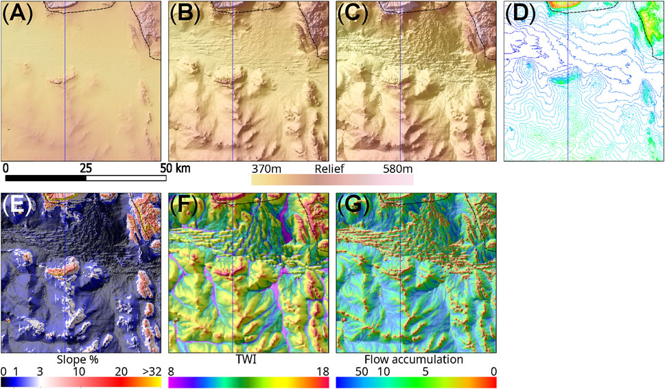
Figure 6. (A) Raw data northwest relief shading 10x vertical exaggeration; (B) Raw data northwest relief shading 100x vertical exaggeration; (C) Raw data aspect shading; (D) Raw data contours at 5-m interval; (E) Raw data slope with aspect shading; (F) TWI of multi-scale resampled data with northwest aspect shading; (G) Flow accumulation of multi-scale resampled data with northwest aspect shading; Tanami Region (black dash); WA-NT border (blue); centred on MGA Zone 52 K 505000E 7815000N, 70 km northwest of Tanami, Northern Territory.
Perhaps the simplest method of identifying a break in slope or significant change in the topography is to look for inflections in contours (Figure 6D). Subtle contour inflections define breaks in slope along open depressions or flats (alluvial plains), and mark the edge of some alluvial fans. Creating slope images is the next stage in producing a map of landforms, the simplest of which is an aspect shaded, multi-scale resampled, colour coded image (Figure 6E), with alternatives using different colour tables and slope classes designed to emphasise landform features.
Topographic Wetness Index
The Topographic Wetness Index (TWI) was developed by Beven and Kirkby (1979), and is commonly used to quantify topographic control on hydrological processes (Sørensen et al., 2006). The TWI was used by Moore et al. (1993) as a first step to guide sampling and model development in unmapped areas. The index was designed for hillslope catenas, so accumulation numbers in flat areas will be very large and the TWI may not be a useful variable. The index is correlated with several regolith attributes, and is useful in identifying hydrological flow paths for geochemical modelling (Figure 6F). GRASS GIS is a geographic information system software suite (GRASS Development Team, 2023) that includes the r.topidx module, which has been used to create a unified predictive model for bedrock and in situ regolith, proximal colluvial slopes, distal colluvial slopes, drainage depressions and stream channels (Figure 7).
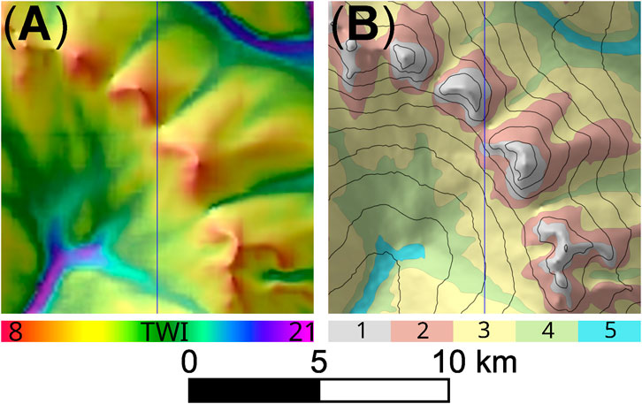
Figure 7. (A) Multi-scale resampled TWI image with northwest illumination; (B) TWI modelled units; 1—in situ regolith, 2—proximal colluvial slopes, 3—distal colluvial slopes, 4—drainage depressions and 5—stream channels; with 5-m topographic contours and northwest illumination; WA-NT border (blue); centred on MGA Zone 52 K 500000E 7773500N, 106 km east of Balgo Community, Western Australia.
Flow Accumulation
The GRASS r.flow module for flow accumulation (Mitasova and Hofierka, 1993; Mitasova et al., 1995) has been designed for modelling erosion on hillslopes. Using flow accumulation images that have a marked directional bias is an effective way of showing the change from downslope drainage in alluvial fans and colluvial slopes, to drainage in the plains perpendicular to hillslopes, regardless of slope values or the presence of clear breaks in slope (Figure 6G). As a mapping method, however, any boundaries determined using flow currently need to be manually crafted as it is being used here for the visualisation of a landform, not the flow accumulation parameters.
Other Methods
Two commonly used techniques for landform mapping are profile curvature (Gozzard and Langford, 2004) and the Multi-resolution Valley Bottom Flatness index (MrVBF; Gallant and Dowling, 2003), both of which have been trialled and found to be unsuitable in areas of very low relief such as the Tanami. A significant break in slope or change in slope can be expressed as a change in the profile curvature image. However, for the Tanami, several algorithms have been applied to both ALOS and TanDEM data, and even the best model was found to be of limited value when compared with extracting breaks in slope using the simple slope and elevation images described in this paper. The MrVBF was used by English et al. (2012) to depict palaeovalley networks, and was therefore considered a valid technique to consider for this study. However, in very flat areas such as the Tanami, MrVBF requires considerable manipulation of the default parameters to get a model that looks even close to the landforms mapped using the simpler combination of elevation, slope, TWI, flow accumulation and spectral response. MrVBF processing is, therefore, not necessarily the best approach for mapping palaeovalleys in this area, given the arbitrary nature of choice of up to six parameters.
Predictive Mapping and Modelling Regolith-Landform Units
The regolith-landform model for the Project Area is based on the identification of landforms, materials and processes primarily using terrain modelling. The regolith is either dominantly in situ or transported, and there are specific landforms associated with each that can be mapped or modelled. The division from in situ regolith through colluvial slopes to drainage depressions and stream channels has not previously been attempted, and accurate mapping of alluvial fans and plains has not previously proved possible in the absence of suitable DEM data. Mapping or modelling these map components (Table 2) has been completed using the following methods, mostly using software modules in the GRASS (GRASS Development Team, 2023) and SAGA (Conrad et al., 2015) software suites:
1. In situ regolith, colluvial slopes, drainage depressions and stream channels: predictive modelling using GRASS r.topidx TWI classification;
2. Alluvial fans: manual interpretation using contours, slope and GRASS r.flow flow accumulation images;
3. Alluvial plains: manual interpretation using contours, slope and TWI images;
4. Pediment: manual interpretation using contours, slope, TWI and spectral images, plus published maps;
5. Playas (closed depressions): modelled using SAGA Basic Terrain Analysis (BTA);
6. Dunes and dunefields: modelled using published data;
7. Palaeovalleys: based on plains, playas and contours;
8. Channel network: modelled using SAGA BTA; and,
9. Drainage basins: published data.
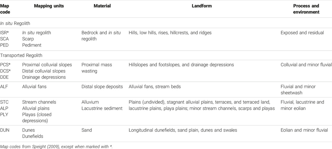
Table 2. Adapted from Hocking et al. (2007) and Wilford and Butrovski (1999).
The TWI algorithm creates an image that has been used to map in situ regolith, colluvial slopes and open depressions (drainage depressions and stream channels), based on a visual examination of the wetness image (Table 3; Figure 7). Apart from stream channels, the TWI modelled areas were removed if overlapped by alluvial fans, alluvial plains, dunes or playas (closed depressions), which all relied on different methodologies for modelling. As closed depressions are geomorphometrically derived, the latter have been chosen to overprint the alluvial fans because the distal material in the alluvial fans may be dominated by later processes active in the depressions, and not dominantly derived by downslope processes that formed the alluvial fan. The alluvial fans are also overlain by stream channels, alluvial plains and dunes.
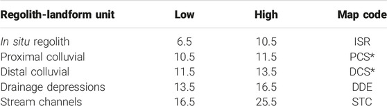
Table 3. TWI modelled regolith-landform units; *hillslopes (HSL) in Speight (2009) have been divided in proximal (PCS) and distal colluvial slopes (DCS).
In situ Regolith ISR
In situ regolith is the primary source of geochemical signatures, and understanding the nature of this source and the proximal dispersion is critical to understanding distal dispersion patterns. In situ regolith is found where transported regolith is thin or absent. There may be thin colluvial, sheetflow or alluvial cover, or degradation of the weathered rock creating a veneer of duricrust or lag. Where well exposed the in situ bedrock material is typically weathered, but usually retains original rock structures and textures. Bedrock and closely related regolith materials are mostly found in areas of high relief, such as escarpments, and on the crests and upper surfaces of low hills and rises. Although there are a few areas with steeper slopes, most of these low hills and rises have slopes less than 3%. Modelled in situ regolith could easily be split into two components based on topography and spectral response. One is spectrally and topographically well defined outcrop, the second is poorly exposed or thinly covered hilltops, some with a spectral signature (duricrust).
Erosional Scarps SCA
Major scarps with slopes over 10% have been extracted as a distinct mapping landform element because they will be the best places to find in situ regolith. The break in slope marking an erosional scarp is usually a sign of headward erosion into the hill and typically located in bedrock exposures. The downslope geochemical pathway from these erosional features will have a strong connection to the material in the scarp.
Proximal and Distal Colluvial Slopes PCS DCS
Proximal colluvial slopes are more likely to include in situ regolith and erosional areas, with less aggradation than the distal colluvial slopes, which will be dominantly aggradational. The aggradational material in these slopes should be colluvium and sheet wash eroded from the surrounding areas, with minor fluvial reworking. Given that the material in colluvial slopes has been derived from proximal upslope in situ regolith, there will be a strong geochemical connection to the source. Understanding the flow paths that contribute the material on these slopes is critical to identifying possibly anomalous sources in the immediate surrounding area. Unlike the large-scale features, such as alluvial fans and plains, dispersion will typically be confined and proximal, giving a very different geochemical dispersion pattern to those landforms with extensive distal dispersion and dilution.
Drainage Depressions DDE
Drainage depressions are one of two open depression (vale) geomorphological types, the other being stream channels (Figure 2B in Speight, 2009). They are characterised by a convex downslope contour pattern, and restricted or absent breaks in slope marking the edge of the landform. This makes mapping much harder and more subjective than for landforms such as fans and plains that have clear, albeit diffuse, breaks in slope. They are important in understanding the movement of material from the source, with a mix of aggradation and channelled erosion. Unlike the large-scale features, such as alluvial fans and plains, dispersion will typically be confined and proximal, giving a very different geochemical dispersion pattern to those landforms with extensive distal dispersion and dilution.
Alluvial Fans ALF
These are places where material has been spread out from a narrow outlet within the adjacent hills and rises to form cone-shaped deposits with a distributary drainage pattern, and these are areas of significant geochemical dispersion. The flow accumulation for fans is radial downslope, contrasting with the orthogonal accumulation on most slopes (colluvium), and the longitudinal accumulation in the axial tributary system of major drainage lines, or radial upslope on hillslopes. This distinctive landform pattern is widespread in the area and was initially mapped using SRTM imagery (Langford, 2008).
There is a distinct topographic high point from which alluvial fans either disgorge through a narrow opening between low hills or rises, or develop from broader stream channels, and together with their characteristic shape this has been used to map their extent. There is not usually a well defined break in slope to aid mapping, so a primary mapping consideration is the divergent radial pattern of contours. The divergence from the source can be broad and extensive, with some alluvial fans up to 20 km long and up to 20 km wide, although the majority are 5–10 km long and wide.
The two resources that have proven to be the best for identifying and manually mapping alluvial fans are elevation contours at 5- or 2-m intervals, and flow accumulation. The contours quickly confirm whether the feature has a radial pattern and a simple point source. The flow direction and pattern is better at reinforcing the interpretation than simple slope, as the images show any radial downslope drainage pattern much more effectively.
Alluvial Plains ALP
Plains are level landforms, although in the Tanami, where nearly everything is level, the term very flat better describes their likely occurrence. This means that only large areas with slopes between 0% and 0.2% are likely to be plains.
As an alluvial plain forms the entire depositional zone in a valley, bounded by hillslopes on either side (English et al., 2012), the simplest method is to identify where there is clear break in slope. A typical 10-km wide plain has slopes dominantly around 0%–0.2%, with adjacent hillslopes mostly 0.2%–1%, so given the scale and small changes in slope, it has not proved to be useful or effective to use geomorphometric analysis to define breaks in slope. Simple visualisation of slope and flow images, aided by assessing changes in 2-m contours, is the chosen method, as contour inflections and decreased contour spacing both indicate breaks in slope. Flow accumulation tends to emphasise landforms that are flat such as alluvial plains and produces the best images. In the Tanami the alluvial plains are largely relict, with little or no active erosion or aggradation.
Pediments PED
Pediments are distinctive types of plain that are underlain by bedrock, and which are gently inclined to level (less than 1%) with very low relief (Speight, 2009). There are pediments in the Project Area, mapped based on structural trends seen in Landsat and other imagery, but none have been identified in the Tanami.
Playas or Closed Depressions PLY
Closed depressions are areas where water could accumulate as they have no apparent outlet channels. Geochemically, these will be areas dominated by accumulation from the surrounding slopes and drainage pathways. The most likely process creating the smaller playas is deflation, with weathering and fluvial erosion in dismembered drainage systems contributing more to the formation of the large-scale depressions (Bourne and Twidale, 2010).
Closed depressions have not previously been mapped as a separate regional-scale landform unit in the Tanami. The digital format of elevation models now provides the basis for a numerical approach to accurately identify and delineate closed depressions (Pardo-Igúzquiza and Dowd, 2021). They may form part of a plain landform pattern, for example, a playa in an alluvial plain, and are being treated here as a distinct and important landform because of their scale, abundance and significance for material accumulation. SAGA BTA (Conrad et al., 2015) has been used to create a model of closed depressions (Planchon and Darboux, 2002), with values that measure the depth of the depression in metres below the surrounding ground.
As the material accumulation in closed depressions is at the lowest point in geochemical dispersion, and comes from a wide spread of sources, sampling in these areas is problematic; the upstream source of the inflow to a playa is a more useful indicator. As sediment that has accumulated in closed depressions has been trapped in close proximity to the adjacent and upstream source, they can be useful for geochemical sampling.
Dunes and Dunefields DUN
A longitudinal dunefield (Speight, 2009) is characterised by a combination of long, narrow sand dunes and wide, flat swales, which are linear, level-floored open depressions excavated by wind, or left relict between the dunes built up by wind. Although the eolian transported material that forms the dunes does not occupy a large area, they are a distinctive feature in the landscape that is important for understanding some aspects of geochemical dispersion.
The map of dunes used in this paper is taken directly from Geoscience Australia topographic data sources (Geoscience Australia, 2006). The mapped dunes in the area are up to 23 km long, and mostly less than 200 m wide in high resolution satellite imagery. However, the lower resolution TanDEM slope data shows them as ridges mostly up to 350 m wide with slopes around 3%. The chosen method for adding dunefields to the regolith-landform map is to take the existing data, with minor edits, and buffer the dunes to 300 m wide, none of which lie in the Tanami.
Stream Channels STC
Stream channels are a type of open depression or vale that sits downslope from a drainage depression (Speight, 2009). They mark a change from downslope material transport to channelled transport away from the adjacent slopes, and are incised into the dominantly aggradational lower slopes. Most historical geological mapping refers to these channels as alluvial, but as they are dominantly erosional, the amount of aggradation will not only be small but also geochemically representative of a much larger part of the immediate catchment relative to the downslope accumulation in colluvial slopes. As erosional landforms they are the youngest features in the area, and cut all other landforms, including dunes.
Drainage Basins and Channel Network
A complete set of catchments and drainage basins is available as Phase 3 Geofabric products (Bureau of Meteorology, 2015), based on improved multi-scale (1:25,000–1:250,000) mapped features and the SRTM 1 arcsecond DEM. Although, for this paper, no use has been made of the very detailed published drainage basins and catchments, using TanDEM data and SAGA BTA to produce a channel network does show differences to the patterns derived from the 1 arcsecond SRTM DEM. Any remapping of catchments using the DEM with a better vertical resolution may produce a more accurate pattern, but is beyond the scope of this paper. The channel network derived from multi-scale resampled elevation using BTA is shown in Figure 8 as a single network with a Strahler number from 3 to 8 (Strahler, 1952), together with the NCB Level1 Drainage Division that represents the highest level of the catchment hierarchy (Bureau of Meteorology, 2015).
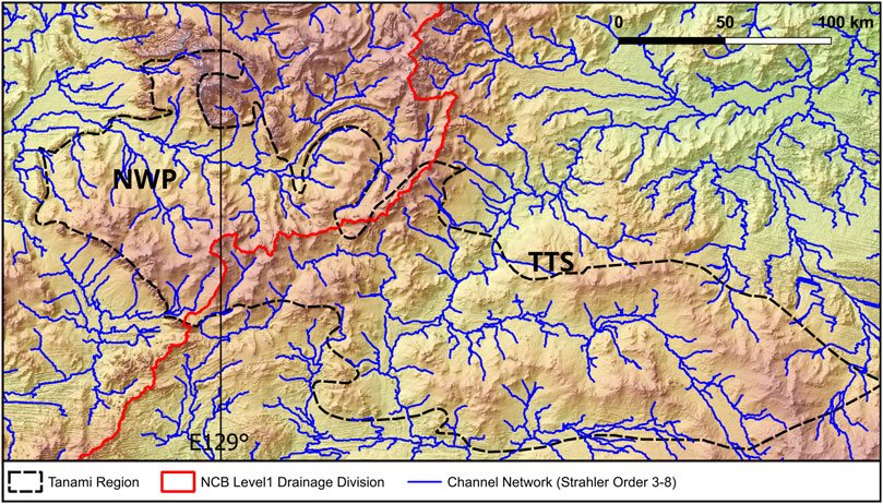
Figure 8. Drainage basins [red; NWP, North Western Plateau; TTS, Tanami-Timor Sea Coast; © Commonwealth of Australia (Bureau of Meteorology, 2015)] covering the Tanami Region, with major stream channels.
Palaeovalleys
Palaeovalleys are found along the alluvial plains and the larger channels connecting some of the plains. They may extend beneath alluvial fans and other slope deposits, but this cannot be determined by surface mapping. In most cases, the WASANT Palaeovalley Map (Bell et al., 2012) represents palaeovalleys as the entire depositional zone between adjoining slopes (English et al., 2012). Wilford (2003) mapped a complex palaeodrainage system that had been preserved in the Granites–Tanami region due to its low relief. For this paper, the likely occurrence of palaeovalleys has been determined by comparing major drainage channels with mapped alluvial plains, and in Figure 9 is shown only as flow directions, which can be compared with both the mapped plains and the published extent of palaeovalleys (WASANT). There are several places where the flow direction changes, where flow ends in closed depressions, or where flow extends in areas not previously identified as palaeovalleys, and as a result the new mapping provides clearer information on material transport paths than the published palaeovalleys.
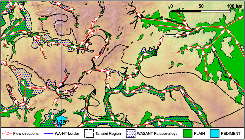
Figure 9. Revised palaeodrainage shown by significant drainage directions on mapped plains and pediment, overlain on WASANT palaeovalleys (Bell et al., 2012).
Results of Interpretation
The new map, which is a combination of classical mapping and geomorphometric modelling, uses the mapping units shown in Table 2 and is shown as Figure 10. Notionally, the mapping scale for the project is 1:250,000, and the appropriate map scale for landform pattern mapping is a minimum width of 750 m (Speight, 2009). For simplicity, this is changed from width to area, with the smallest unit area preserved in this mapping of approximately 450,000 m2, making the map more comparable to the commonly available 1:250,000-scale mapping. Two mapping examples below have been selected to show the full level of detail in contrasting areas, with clear landform patterns in one, and poor landform definition in the other.
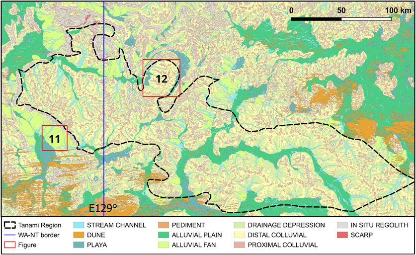
Figure 10. Regolith-landform map of the Tanami Region and surrounding area, produced at 1:250,000-scale.
Mapping Example 1—Low Hills and Alluvial Fans
The first of two examples is focused on an area with some clear and distinctive landforms, the interpretation of which has a direct bearing on the interpretation of material transport and geochemistry. Located in the west of the Tanami and dominantly within the adjacent Birrindudu Region, this case study area has an elevation range from 370 m in the southwest to 500 m in the northeast. The topographic image (Figure 11A) shows a line of low hills to the northeast, an extensive playa to the southwest, and alluvial fans between the two, including one that is 20 km long and up to 20 km wide; the radial contour pattern is the clearest confirmation of the fans. The Landsat TM image (Figure 11B) shows good lithological detail in the low hills, and confirms the radial distribution of material in the large fan, although not extending to the full extent of the landform. The slope image (Figure 11C) provides a better definition of the low hills, with slopes mostly over 2% and up to 20%, with distinct breaks in slope at the margins. The alluvial fans have slopes between 0.2% and 0.4%, and the playa mostly 0%–0.1%, but up to 0.2%, potentially making it difficult to differentiate the fans from the playas. The TWI image (Figure 11D) provides a clear indication of the alluvial channels at the margins of the fans, and the flow accumulation image (Figure 11E) not only shows the radial pattern typical of alluvial fans but also a clear margin between the playa and the fans.
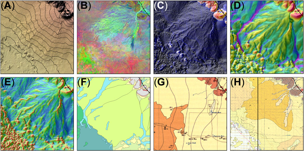
Figure 11. (A) Topographic relief northwest shading with 5-m contours; (B) Landsat DS754; (C) Slope northwest aspect-shading; (D) Multi-scale TWI northwest aspect-shading; (E) Multi-scale flow accumulation northwest aspect-shading; (F) Final regolith-landform map; (G) 1:250,000-scale mapping (Crowe et al., 1977); (H) 1:100,000-scale mapping (Eacott and de Souza Kovacs, 2015a; 2015b); 25 km × 25 km area centred on MGA Zone 52 K 450800E 7758400N, 60 km east of Balgo Community, Western Australia; Tanami Region (black dash).
The final map (Figure 11F) correlates well with all the features visible in shaded topography, contours, slope, TWI and flow accumulation, and to a lesser extent with the Landsat. The overlap between the alluvial fans and closed depressions is about 0.5–1 km, and has been mapped in favour of the morphometrically modelled closed depressions where material transport will be currently active.
There are two published geological maps covering the case study; Crowe et al. (1977) (Figure 11G), and 1:100,000-scale mapping by Eacott and de Souza Kovacs (2015a), Eacott and de Souza Kovacs (2015b) (Figure 11H). There is good agreement on the interpretation of in situ regolith from the oldest mapping to the new map, which would be expected based on the distinctive topography and spectral response. The oldest published map (Crowe et al., 1977) is dominated by sand plain and calcrete, in stark contrast to the new mapping in this paper. A partial alluvial fan identified in more recent published mapping (Eacott and de Souza Kovacs, 2015a; Eacott and de Souza Kovacs, 2015b) contrasts with numerous fans identified in the new mapping. As these fans are not sourced from the low hills, but from within the Tanami to the east, this is a significant factor in understanding geochemical dispersion patterns. This contrasts with areas where well defined in situ regolith is the source for material in the colluvial slopes, highlighting the importance of distinguishing fans from simple slopes across the Tanami.
Mapping Example 2—Very Low Relief Terrain
The second example is focused on an area with poor landform definition, which is typical in most of the Tanami. The recognition of subtle landforms is needed not only to model material transport, but also to better identify the likelihood of in situ or shallow bedrock not previously identified. Located within the northwest of the Tanami, and surrounded by low hills and ridges in the adjacent Birrindudu Region, this case study area has an elevation range from 390 m to 460 m.
The topographic image (Figure 12A) shows a number of north and west trending hillcrests, with extensive playas and closed depressions to the east and west. The shaded relief pattern is the clearest confirmation of the shape of these ridges and intervening open depressions. The Landsat TM image (Figure 12B) shows a uniform spectral response across the elevated areas and distinctive responses in the alluvial channels, playas and closed depressions. Based on the response, the low hills are possibly dominated by eolian quartz with little or no ferruginous material (Gozzard, 2004), although field mapping would be needed to accurately correlate response and regolith material. The slope image (Figure 12C) confirms that the dominant slopes are <0.7%, which would mean the area is classified as level (Speight, 2009). There is, however, a clear difference between the slopes on the low hills (0.3%–1%), and the ridge lines, open and closed depressions, and playas (0%–0.2%). The TWI image (Figure 12D) provides a clear indication of the alluvial channels in the open depressions, and the flow accumulation image (Figure 12E) shows both the dendritic pattern typical of downslope flow, and the mixed pattern typical of the playas and closed depressions. The final map (Figure 12F) correlates well with all the features visible in shaded topography, contours, slope, TWI and flow accumulation, and the Landsat image provides good discrimination of material types.
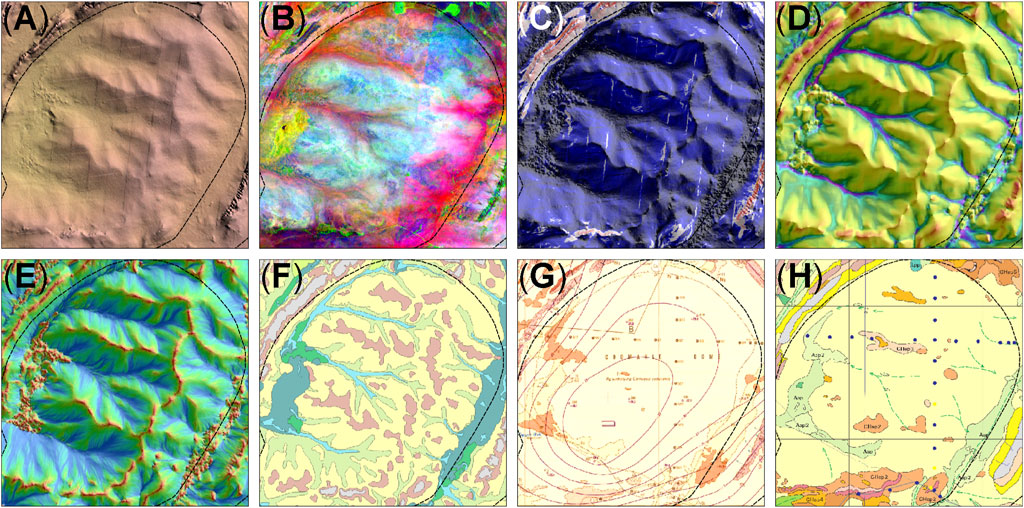
Figure 12. (A) Topographic relief northeast shading with 5-m contours; (B) Landsat DS754; (C) Slope northeast aspect-shading; (D) Multi-scale TWI northeast aspect-shading; (E) Multi-scale flow accumulation northeast aspect-shading; (F) Final regolith-landform map; (G) 1:250,000-scale mapping (Blake et al., 1975); (H) 1:500,000-scale mapping (Wilford and Butrovski, 1999); 37 km × 37 km area centred on MGA Zone 52 K 557500E 7818500N, 30 km northwest of Tanami, Northern Territory; Tanami Region (black dash).
There are two published geological maps covering the case study; Blake et al. (1975) at 1:250,000-scale (Figure 12G), and Wilford and Butrovski (1999) at 1:500,000-scale (Figure 12H). The oldest published map (Blake et al., 1975) is dominated by eolian and piedmont sand and gravel, with minor alluvial and calcrete deposits; laterite capping is only mapped on the low hills to the south. The later map (Wilford and Butrovski, 1999) shows this area as mostly colluvial deposits with some alluvial channel deposits on low relief sheet flood colluvial plains. There are also minor erosional plains, and eolian sand reworked by sheetflow (process), with some patches of sand and gravel over ferruginous saprolite or duricrust. When compared with the new map and underlying images, there is likely to be more near in situ material on the numerous ridges than is shown in the historical mapping, and the clear identification of colluvial slopes provides a better understanding of material transport away from sources not previously identified.
Discussion
Both manual mapping and geomorphometric analysis have been used to extract an interpretation from DEM data and a range of derived images. MacMillan et al. (2000) described the three major problems for an automated landform classification algorithm for identifying different types of landscapes using DEMs as follow:
• Selecting and computing an appropriate suite of terrain derivatives from DEM data.
• Identifying an appropriate number of meaningful different landform classes and describing their salient or defining characteristic.
• Selecting and applying a classification procedure capable of using the available terrain derivatives to produce the required classes.
The Project Area mapping and these case studies in and around the Tanami have effectively addressed all three problems:
• Using TanDEM data, the best terrain derivatives have been established as relief, slope, TWI and flow accumulation, with a strong preference for visualisation as a mapping tool.
• The suitably processed data and imagery have been used to create and define eleven meaningful classes; in situ regolith, scarps, proximal and distal colluvial slopes, drainage depressions, stream channels, alluvial fans, alluvial plains and pediments, closed depressions, and dunes and dunefields.
• The procedure has been varied according to the landform being assessed, ranging from geomorphometric classification using TWI to manual mapping using relief, slope and flow accumulation. In addition, adapting existing map data for dunes has created an effective landform filter, and validation of the regolith-landform model has been undertaken using remotely sensed imagery and published maps.
Conclusion
A major challenge for mineral exploration geologists is the development of a transparent and reproducible approach to targeting exploration efforts, particularly at the regional-to camp-scales, in terranes under difficult cover where exploration and opportunity costs are high (Joly et al., 2012). Exploration targeting using geochemistry can be biased to areas of in situ regolith, however potential high value targets identified by Joly et al. (2012) lie largely under cover, and this work provides greater clarity on the landforms and material distribution in areas of transported regolith.
A region like the Tanami has in the past been seen only as dominated by flat sand plain, because superficially that is an accurate description (Wells and Billiluna, 1962a; Wells and Lucas, 1962b; Blake et al., 1972; Blake et al., 1975; Hodgson, 1975; Hodgson, 1976; Crowe et al., 1977; Hulleat, 1978; Offe and Kenewell, 1978; Blake et al., 1979). The recognition by Wilford and Butrovski (1999) and others that major palaeodrainage and other landform complexities were important aspects of the region that would influence models and mapping was hindered at the time by a lack of good elevation data. Using conventional landform classification (Speight, 2009) the vast majority of the area has slopes of less than 1%, so is level, and the dominant material at the surface is eolian sand. Using traditional mapping methods, even with the addition of spectral imagery, this is a reasonable interpretation. However, with high resolution elevation data, this view of the landscape becomes untenable. This paper has shown that the perception that a complex set of landform patterns does not exist can be overturned by using a dataset that clearly shows that the landforms are real and mappable. The Tanami has a complex and varied set of landforms ranging from low hills and escarpments to alluvial plains and playas, all with a partial cover of eolian sand and dunes.
No amount of complex processing will extract landforms from the data if the initial choice of data is not appropriate, which can be a function of both resolution and measurement type. Following a review of available DEM data, the presumption that the Tanami is not only level but also featureless has been tested using TanDEM data and shown to be false. This paper shows that TanDEM satellite-derived elevation data are the most appropriate to use in areas of very low relief, such as the Tanami, for regional-scale regolith-landform mapping.
This paper has highlighted the difficulty not only of identifying datasets suitable for creating regolith-landform maps but also the wide variety of choices for creating the map units, ranging from simple visualisation to manipulating complex algorithms. Underlying the study is the desirability of an outcome oriented rather than process oriented approach. At all stages, the outcome is pre-determined to varying degrees of certainty based on the simplest visual estimation using relief and slope. Any subsequent modifications to the input data, derived imagery or additional processes are all designed to improve on the initial expected outcome.
Modelling the data and images has produced a regolith-landform map for the Tanami that would have been impossible without suitable topographic data. This work has demonstrated that the choice of a suitable elevation dataset for regional mapping, such as TanDEM, and creative manipulation of those data to create images, will effectively elucidate the landscape in areas of very low relief. The underlying philosophy is not restricted to areas of very low relief. The temptation in areas of higher relief is to assume that the visually obvious topography does not hide more complex subdued or subtle landform pattern. The techniques described can be applied in any area, with careful choice of data input and manipulation designed to enhance features that may otherwise be overlooked.
Areas of very low relief and slopes that are typically seen as level or near level, such as the Tanami, possess a wealth of landform diversity that is directly relevant not only to the planning and interpretation of geochemical survey results, but also to other land use studies. A failure to delve deeper into the geomorphology of an area of very low relief, and to presume that there is a uniformity in landform, processes and materials, has resulted in the Tanami mostly being seen as a near uniform sand plain, with few upstanding features. Using SRTM data initially (Langford, 2007; Langford, 2015) and now TanDEM data demonstrates how a variety of methods can now be applied to produce a robust regolith-landform map. As technology improves, there is also an opportunity for all the map components to be geomorphometrically extracted, but for now a mixture of classical and geomorphometric techniques has been shown in this paper to produce the best predictive regolith-landform map.
Data Availability Statement
Publicly available datasets were analyzed in this study. This data can be found here: https://zenodo.org/records/10466843, SRTM Void Filled [Digital Object Identifier (DOI) number: /10.5066/F7F76B1X] SRTM 1 Arc-Second Global [Digital Object Identifier (DOI) number: /10.5066/F7PR7TFT], https://zenodo.org/records/10466927.
Author Contributions
The author confirms being the sole contributor of this work and has approved it for publication.
Funding
The author declares that no financial support was received for the research, authorship, and/or publication of this article.
Conflict of Interest
The author declares that the research was conducted in the absence of any commercial or financial relationships that could be construed as a potential conflict of interest.
Publisher’s Note
All claims expressed in this article are solely those of the authors and do not necessarily represent those of their affiliated organizations, or those of the publisher, the editors and the reviewers. Any product that may be evaluated in this article, or claim that may be made by its manufacturer, is not guaranteed or endorsed by the publisher.
Acknowledgments
We acknowledge the past and present Traditional Owners of Ngarti, Pintupi and Warlpiri country. Inkscape™ and Quantum software were used to create the figures (Quantum GIS Development Team, 2017; The Inkscape Project, 2023).
References
Bagas, L., Anderson, J. A. C., and Bierlein, F. P. (2009). Palaeoproterozoic Evolution of the Killi Killi Formation and Orogenic Gold Mineralization in the Granites–Tanami Orogen, Western Australia. Ore Geol. Rev. 35, 47–67. doi:10.1016/j.oregeorev.2008.09.001
Bain, J. H. C., and Draper, J. J. (1998). “North Queensland Geology,” in AGSO Bulletin, 240 (Canberra: Australian Geological Survey Organisation).
Bell, J. G., Kilgour, P. L., English, P. M., Woodgate, M. F., and Lewis, S. J. (2012). WASANT Palaeovalley Map – Distribution of Palaeovalleys in Arid and Semi-Arid WA-SA-NT. 1st ed.
Beven, K. J., and Kirkby, M. J. (1979). A Physically Based, Variable Contributing Area Model of Basin Hydrology/Un Modèle à Base Physique de Zone d’appel Variable de l’hydrologie du Bassin Versant. Hydrol. Sci. Bull. 24, 43–69. doi:10.1080/02626667909491834
Blake, D. H., Hodgson, I. M., and Muhling, P. C. (1979). Geology of the Granites-Tanami Region, Northern Territory and Western Australia. Bureau Mineral Resour. Geol. Geophys. Aust. Canberra, Bull. 197, 46pp. plus map.
Blake, D. H., Hodgson, I. M., and Smith, P. A. (1972). Geology of the Birrindudu and Tanami 1: 250,000 Sheet Areas, Northern Territory. Report on the 1971 Field Season. Canberra, Australia: Bureau of Mineral Resources, Geology and Geophysics. Record 92. 135pp plus maps.
Blake, D. H., Hodgson, I. M., and Smith, P. A. (1975). Tanami, Northern Territory, Sheet SE/52-15. Australia 1:250,000 Geological Series. Bureau of Mineral Resources. Australia, Canberra: Geology and Geophysics.
Blake, D. H., and Kilgour, B. (1998). Geological Regions of Australia, 1:5,000,000-Scale. Canberra: Geoscience Australia.
Bourne, J. A., and Twidale, C. R. (2010). Playas of Inland Australia. Cad. Lab. Xeolóxico Laxe Coruña 35, 71–98.
Bureau of Meteorology (2015). Australian Hydrological Geospatial Fabric (Geofabric) Product Guide Version 3.0, 48pp. Australia: Australian Government.
Carroll, D., and Morse, M. P. (1996). A National Digital Elevation Model for Resource and Environmental Management. Cartography 25, 43–49. doi:10.1080/00690805.1996.9714031
Chan, R. A. (1988). Regolith Terrain Mapping for Mineral Exploration in Western Australia in Applied Geomorphological Mapping: Methodology by Example. Z. für Geomorphol. Suppl. 68, 205–211.
Christian, C. S., Stewart, G. A., Nokes, L. C., and Blake, S. T. (1953). “General Report on Survey of Katherine-Darwin Region, 1946,” in Land Research Series 1, 156pp Plus Plates (Australia, Melbourne: Commonwealth Scientific and Industrial Research Organisation).
Conrad, O., Bechtel, B., Bock, M., Dietrich, H., Fischer, E., Gerlitz, L., et al. (2015). System for Automated Geoscientific Analyses (SAGA) V. 2.1.4. Geosci. Model Dev. 8, 1991–2007. doi:10.5194/gmd-8-1991-2015
Crispe, A., Vandenberg, L., and Green, M. (2005). Mount Solitaire, Northern Territory. 2nd ed. Darwin: Northern Territory Geological Survey. 1:250,000-scale geological map series, SF 52-04.
Crispe, A. J., Vandenberg, L. C., and Scrimgeour, I. R. (2007). Geological Framework of the Archean and Paleoproterozoic Tanami Region, Northern Territory. Miner. Deposita 42, 3–26. doi:10.1007/s00126-006-0107-1
Crowe, R., Muhling, P. C., Blake, D. H., and Walton, D. G. (1977). Lucas, Western Australia. Australia, Canberra: Geology and Geophysics. Sheet SE/52-2, 1:250,000 Geological Map Series. Bureau of Mineral Resources.
Diaby, H. A., Kouamé, F., Saley, B., and Ansah, K. O. (2023). Automated Mapping of Regolith Units with Support Vector Machine and Artificial Neural Network Using Data from Landsat-8 OLI, ALOS PALSAR DEM, and Sentinel-1A Radar Images: The Case of the Sissingué Gold Project, Northern Côte d’Ivoire. Int. J. Remote Sens. 44, 7126–7155. doi:10.1080/01431161.2023.2282406
Dobos, E., Daroussin, J., and Montanarella, L. (2010). A Quantitative Procedure for Building Physiographic Units Supporting a Global SOTER Database. Foldr. Ertesito/Hungarian Geogr. Bull. 59, 181–205.
Eacott, G. R., and de Souza Kovacs, N. (2015a). Kearney, WA Sheet 4557, 1. Western Australia: Geological Survey of. 100,000 Geological Series.
Eacott, G. R., and de Souza Kovacs, N. (2015b). Lewis, WA Sheet 4657, 1. Western Australia: Geological Survey of, 100. 000 Geological Series.
Earth Resources Observation And Science (EROS) Center (2017b). Shuttle Radar Topography Mission (SRTM) 1 Arc-Second Global. doi:10.5066/F7PR7TFT
Earth Resources Observation And Science (EROS) Center (2017a). Shuttle Radar Topography Mission (SRTM) Void Filled. doi:10.5066/F7F76B1X
Eggleton, R. A. (2000). The Regolith Glossary: Surficial Geology, Soils and Landscape (Melbourne: CSIRO Publishing).
English, P., Lewis, S., Bell, J., Wischusen, J., Woodgate, M., Bastrakov, E., et al. (2012). Water for Australia’s Arid Zone—Identifying and Assessing Australia’s Palaeovalley Groundwater Resources: Summary Report. Canberra: National Water Commission.
Gallant, J. C., and Dowling, T. I. (2003). A Multiresolution Index of Valley Bottom Flatness for Mapping Depositional Areas. Water Resour. Res. 39, 1347–1360. doi:10.1029/2002wr001426
Geoscience Australia Australian National University, and Fenner School of Environment and Society (2008). GEODATA 9 Second DEM and D8 Digital Elevation Model Version 3 and Flow Direction Grid 2008. User Guide. Canberra, ACT: Geoscience Australia, 45pp.
Geoscience Australia (2006). GEODATA TOPO 250K Series 3 (Shape File Format). Canberra: Geoscience Australia.
Gozzard, J. R. (2004). “Part 2: Predictive Regolith-Landform Mapping,” in SEG 2004 Workshop 1, How to look at, in and through the regolith for efficient predictive mineral discoveries, workshop notes, Western Australia, Perth, SEG 2004, November 10-11, 2004, 163p.
Gozzard, J. R., and Langford, R. L. (2004). “Remote Sensing and High-Resolution Landscape Models in Predictive Geological Mapping,” in 12th Australasian Remote Sensing and Photogrammetry Conference, Fremantle, 18–22 October 2004.
Gozzard, J. R., and Tapley, I. J. (1994). “Improved Regolith–Landform Mapping Using Landsat TM Imagery as an Aid to Mineral Exploration in the Lawlers District, North-Eastern Goldfields Region, Western Australia,” in Proceedings of the 7th Australasian Remote Sensing Conference, Melbourne, Australia, 1-4 March 1994.
GRASS Development Team (2023). Geographic Resources Analysis Support System (GRASS) Software. Open Source Geospatial Found. Version 8.3. doi:10.5281/zenodo.5176030
GSWA (2009). West Tanami Project: Geology of the Granites - Tanami Orogen. GSWA Open Day 2009 Poster. Available at: https://dmpbookshop.eruditetechnologies.com.au/product/west-tanami-gswa-feb-09.do.
Hendrickx, M. A., Slater, K., Crispe, A. J., Dean, A. A., Vandenberg, L. C., and Smith, J. B. (2000). Palaeoproterozoic Stratigraphy of the Tanami Region: Regional Correlations and Relation to Mineralisation—Preliminary Results. North. Territ. Geol. Surv. Rec. 13, 71pp.
Hocking, R. M., Langford, R. L., Thorne, A. M., Sanders, A. J., Morris, P. A., Strong, C. A., et al. (2007). A Classification System for Regolith in Western Australia (March 2007 Update). East Perth, Western Australia: Western Australia Geological Survey Record. Available at: https://dmpbookshop.eruditetechnologies.com.au/product/a-classification-system-for-regolith-in-western-australia-march-2007-update.do.
Hodgson, I. M. (1975). Tanami, Northern Territory, Sheet SE/52-15. 1:250,000 Geological Series Explanatory Notes. Bureau of Mineral Resources. Australia, Canberra: Geology and Geophysics, 17pp.
Hodgson, I. M. (1976). The Granites, Northern Territory, Sheet SF/52-3. 1:250,000 Geological Series Explanatory Notes. Bureau of Mineral Resources. Australia, Canberra: Geology and Geophysics, 15pp.
Hou, B., Frakes, L. A., Sandiford, M., Worrall, L., Keeling, J., and Alley, N. F. (2008). Cenozoic Eucla Basin and Associated Palaeovalleys, Southern Australia — Climatic and Tectonic Influences on Landscape Evolution, Sedimentation and Heavy Mineral Accumulation. Sediment. Geol. 203, 112–130. doi:10.1016/j.sedgeo.2007.11.005
Huleatt, M. B. (1978). Tanami East, Northern Territory, Sheet SE/52-16. 1:250,000 Geological Series Explanatory Notes. Bureau of Mineral Resources. Australia, Canberra: Geology and Geophysics, 13pp.
Huston, D. L., Vandenberg, L., Wygralak, A. S., Mernagh, T. P., Bagas, L., Crispe, A., et al. (2007). Lode–gold Mineralization in the Tanami Region, Northern Australia. Miner. Deposita 42, 175–204. doi:10.1007/s00126-006-0106-2
Jiang, Z., Mallants, D., Peeters, L., Gao, L., Soerensen, C., and Mariethoz, G. (2019). High-Resolution Paleovalley Classification from Airborne Electromagnetic Imaging and Deep Neural Network Training Using Digital Elevation Model Data. Hydrol. Earth Syst. Sci. 23, 2561–2580. doi:10.5194/hess-23-2561-2019
Joly, A., Porwal, A., and McCuaig, T. C. (2012). Exploration Targeting for Orogenic Gold Deposits in the Granites-Tanami Orogen: Mineral System Analysis, Targeting Model and Prospectivity Analysis. Ore Geol. Rev. 48, 349–383. doi:10.1016/j.oregeorev.2012.05.004
Knight, R., Smith, R., Asch, T., Abraham, J., Cannia, J., Viezzoli, A., et al. (2018). Mapping Aquifer Systems with Airborne Electromagnetics in the Central Valley of California. Groundwater 56, 893–908. doi:10.1111/gwat.12656
Krieger, G., Moreira, A., Fiedler, H., Hajnsek, I., Werner, M., Younis, M., et al. (2007). TanDEM-X: A Satellite Formation for High-Resolution SAR Interferometry. IEEE Trans. Geoscience Remote Sens. 45, 3317–3341. doi:10.1109/tgrs.2007.900693
Langford, R. L. (2007). Regolith Terrain Mapping in the Tanami. GSWA 2007 Ext. Abstr. Promot. Prospect. West. Aust. 2, 3–4. Geological Survey of Western Australia, Record.
Langford, R. L. (2008). “Regolith Landform Mapping in the Tanami,” in Visualising Landscape Evolution with SRTM Data (Perth, Western Australia: AESC presentation).
Langford, R. L. (2015). Temporal Merging of Remote Sensing Data to Enhance Spectral Regolith, Lithological and Alteration Patterns for Regional Mineral Exploration. Ore Geol. Rev. 68, 14–29. doi:10.1016/j.oregeorev.2015.01.005
MacMillan, R., Pettapiece, W., Nolan, S., and Goddard, T. (2000). A Generic Procedure for Automatically Segmenting Landforms into Landform Elements Using DEMs, Heuristic Rules and Fuzzy Logic. Fuzzy sets Syst. 113, 81–109. doi:10.1016/s0165-0114(99)00014-7
Mitášová, H., and Hofierka, J. (1993). Interpolation by Regularized Spline with Tension: II. Application to Terrain Modeling and Surface Geometry Analysis. Math. Geol. 25, 657–669. doi:10.1007/BF00893172
Mitášová, H., Mitas, L., Brown, W. M., Gerdes, D. P., Kosinovsky, I., and Baker, T. (1995). Modelling Spatially and Temporally Distributed Phenomena: New Methods and Tools for GRASS GIS. Int. J. Geogr. Inf. Syst. 9 (4), 433–446. doi:10.1080/02693799508902048
Moore, I. D., Gessler, P. E., Nielsen, G. A., and Peterson, G. A. (1993). Soil Attribute Prediction Using Terrain Analysis. Soil Sci. Soc. Am. J. 57, 443–452. doi:10.2136/sssaj1993.03615995005700020026x
Moreira, A., Krieger, G., Hajnsek, I., Hounam, D., Werner, M., Riegger, S., et al. (2004). TanDEM-X: A TerraSAR-X Add-On Satellite for Single-Pass SAR Interferometry. IGARSS 2004. 2004 IEEE Int. Geoscience Remote Sens. Symposium 2, 1000–1003. doi:10.1109/IGARSS.2004.136857
Mote, T. I., Brimhall, G. H., Tidy-Finch, E., Muller, G., and Carrasco, P. (2001). Application of Mass-Balance Modeling of Sources, Pathways, and Sinks of Supergene Enrichment to Exploration and Discovery of the Quebrada Turquesa Exotic Copper Orebody, El Salvador District, Chile. Econ. Geol. 96, 367–386. doi:10.2113/gsecongeo.96.2.367
Mulligan, A. E., Evans, R. L., and Lizarralde, D. (2007). The Role of Paleochannels in Groundwater/seawater Exchange. J. Hydrology 335, 313–329. doi:10.1016/j.jhydrol.2006.11.025
Offe, L. A., and Kennewell, P. J. (1978). Mount Solitaire, Northern Territory, Sheet SF/52-4, 1:250,000 Geological Series Explanatory Notes. Bureau of Mineral Resources. Australia, Canberra: Geology and Geophysics, 14pp.
Ollier, C. D. (1977). “Early Landform Evolution,” in Australia: A Geography. Editor D. N. Jeans (Sydney, Australia: Sydney University Press), 85–98.
Pain, C., Chan, R., Craig, M., Gibson, D., Ursem, P., and Wilford, J. (2000). RTMAP Regoith Database Field Book and Users Guide. Australia: Cooperative Research Centre for Landscape Evolution and Mineral Exploration, Canberra ACT. (Second Edition) (CRC LEME Report No. 138) 2601.
Pain, C. F. (2008). Field Guide for Describing Regolith and Landforms. Australia, WA, Bentley: CRC LEME, 108.
Pain, C. F., Chan, R., Craig, M., Gibson, D., Kilgour, P., and Wilford, J. (2007). RTMAP Regolith Database Field Book and Users Guide. 2nd ed. Bentley, Western Australia: CRC LEME Open File Report, 92pp.
Pardo-Igúzquiza, E., and Dowd, P. A. (2021). The Mapping of Closed Depressions and its Contribution to the Geodiversity Inventory. Int. J. Geoheritage Parks 9, 480–495. doi:10.1016/j.ijgeop.2021.11.007
Planchon, O., and Darboux, F. (2002). A Fast, Simple and Versatile Algorithm to Fill the Depressions of Digital Elevation Models. Catena 46, 159–176. doi:10.1016/S0341-8162(01)00164-3
Plumb, K. A., Ahmad, M., and Wygralak, A. S. (1990). Mid-Proterozoic Basins of the North Australian Craton: Regional Geology and Mineralisation. Geol. mineral deposits Aust. P. N. G. 1, 881–902.
Quantum GIS Development Team (2017). Quantum GIS Geographic Information System. Switzerland: Open Source Geospatial Foundation Project.
Reid, N., Hill, S. M., and Lewis, D. M. (2005). “Tanami Geobotany and Biogeochemistry: Towards its Characterisation, Role in Regolith Evolution and Implications for Mineral Exploration,” in Regolith 2005 – Ten Years of CRC LEME. Editor I. C. Roach (Bentley, Western Australia: CRC LEME), 256–259. Available at: http://crcleme.org.au/Pubs/Monographs/regolith2005/Reid_et_al.pdf.
Samadder, R. K., Kumar, S., and Gupta, R. P. (2011). Paleochannels and Their Potential for Artificial Groundwater Recharge in the Western Ganga Plains. J. Hydrology 400, 154–164. doi:10.1016/j.jhydrol.2011.01.039
Slater, K. R. (2000a). Tanami 1:250,000 Integrated Interpretation of Geophysics and Geology. Edition 1. Darwin, Australia: Northern Territory Geological Survey.
Slater, K. R. (2000b). The Granites SF 52-3 1:250,000 Integrated Interpretation of Geophysics and Geology. Edition 1. Darwin, Australia: Northern Territory Geological Survey.
Smith, M. E., Lovett, D. R., Pring, P. I., and Sando, B. G. (1998). Dead Bullock Soak Gold Deposits. Aust. IMM Monogr. 22, 449–460.
Sørensen, R., Zinko, U., and Seibert, J. (2006). On the Calculation of the Topographic Wetness Index: Evaluation of Different Methods Based on Field Observations. Hydrol. Earth Syst. Sci. 10, 101–112. doi:10.5194/hess-10-101-2006
Speight, J. G. (2009). “Landform,” in National Committee on Soil and Terrain, 2009. Australian Soil and Land Survey Field Handbook. 3rd ed.) (Melbourne: CSIRO Publishing), 15–72.
Stewart, G. A., and Perry, R. A. (1953). “Part VII. The Land Systems of the Townsville–Bowen Region,” in Survey of Townsville–Bowen Region, 1950. Land Research Series. Editors G. S. Christian, S. J. Paterson, R. A. Perry, R. O. Slatyer, G. A. Stewart, and D. M. Traves (Australia, Melbourne: Commonwealth Scientific and Industrial Research Organization), 2, 55–68.
Strahler, A. N. (1952). Hypsometric (Area-Altitude) Analysis of Erosional Topography. Geol. Soc. Am. Bull. 63, 1117. doi:10.1130/0016-7606(1952)63[1117:HAAOET]2.0.CO;2
Tapley, I. J., and Gozzard, J. R. (1994). “Landsat Thematic Mapper Processing Techniques for Regolith-Landform Mapping in the Eastern Goldfields Region of Western Australia,” in Proceedings of the 7th Australasian Remote Sensing Conference, Melbourne, Australia, 1-4 March 1994.
The Inkscape Project (2023). Inkscape. Available at: https://inkscape.org.
Vandenberg, L., and Crispe, A. (2014). The Granites. Northern Territory. 2nd ed. Darwin: Northern Territory Geological Survey. 1:250,000 geological map series, SF 52-03.
Wells, A. T., and Billiluna, W. A. (1962a). 4-Mile Geological Series, Sheet E/52-14. Bureau Mineral Resour. Geol. Geophys. Aust. Canberra, Explan. Notes 24, 12pp.
WellsLucas, A. T. W. A. (1962b). 4-Mile Geological Series, Sheet F/52-2. Bureau Mineral Resour. Geol. Geophys. Aust. Canberra, Explan. Notes 25, 14pp.
Wilford, J. R. (1995). Airborne Gamma-Ray Spectrometry as a Tool for Assessing Relative Landscape Activity and Weathering Development of Regolith, Including Soils. AGSO Res. Newsl. 22, 12–14.
Wilford, J. R. (2003). Granites–Tanami Region, Northern Territory. Canberra, ACT, Australia: CRC LEME, 1–5.
Wilford, J. R., and Butrovski, D. (1999). Granites Tanami Regolith-Landform Series Special Edition, 1:500,000 Map Scale. Canberra: CRC LEME.
Wilford, J. R., and Butrovski, D. (2000). Customised Regolith Maps Incorporate Hydrologic Modelled Attributes for Geochemical Exploration. AGSO Res. Newsl. 33, 21–23.
Wood, J. (1996). “The Geomorphological Characterisation of Digital Elevation Models,” (UK: University of Leicester), 466pp. PhD Thesis.
Keywords: spaceborne radar, radar imaging, digital elevation models, remote sensing, geomorphometry, regolith-landform
Citation: Langford RL (2024) Geochemical Pathways Defined by Predictive Regolith-Landform Models Using TanDEM-X Data in the Tanami Region, Australia. Earth Sci. Syst. Soc. 4:10111. doi: 10.3389/esss.2024.10111
Received: 29 January 2024; Accepted: 12 April 2024;
Published: 23 May 2024.
Edited by:
Shay Mullineaux, Queen’s University Belfast, United KingdomReviewed by:
Colin Pain, Sevilla University, SpainAlastair Ruffell, Queen’s University Belfast, United Kingdom
Copyright © 2024 Langford. This is an open-access article distributed under the terms of the Creative Commons Attribution License (CC BY). The use, distribution or reproduction in other forums is permitted, provided the original author(s) and the copyright owner(s) are credited and that the original publication in this journal is cited, in accordance with accepted academic practice. No use, distribution or reproduction is permitted which does not comply with these terms.
*Correspondence: Richard Llewellyn Langford, richard.langford@gmx.com