 W. Brian Whalley
- Department of Geography, University of Sheffield, Sheffield, United Kingdom
The essential aspects of Gore’s “Digital Earth” concept include “georeferenced” data. This paper is concerned with establishing the need for a standardised and common form to locate points on the earth’s surface. Rather than a degree, minute, second (dms) system for latitude/longitude location, a decimal degree system, formatted as a comma separated variable tuple in square brackets, [dLL], is advocated. Values, to an appropriate number of decimal places, can be inserted in text to be computer searchable. The [dLL] also becomes metadata for a data set or as an index in databases or identifiers for images. Various uses of this system are illustrated. The [dLL] allows data to become more “open” via the FAIR data principles: findability, accessibility, interoperability, and reusability. Wider use of [dLL] in the earth sciences is fundamental to collaboration with other disciplines, especially Critical Zone Science. The general use of [dLL] geolocation can be exploited in a wide variety of data analytical methodologies, some of which are outlined, and in earth science and environmental data situations.
Introduction
In a talk in 1998, then US Vice President Al Gore indicated that, “We have an unparalleled opportunity to turn a flood of raw data into understandable information about our society and our planet” (Gore, 1999). His suggestion was to build a Digital Earth that would help tame this inundation and “provide a mechanism for users to navigate and search for geospatial information—and for producers to publish it.” Gore also noted that, “The hard part of taking advantage of this flood of geospatial information will be making sense of it—turning raw data into understandable information.” Here I revisit Digital Earth with specific focus on providing better geolocated and georeferenced data. In particular, I explore ways to produce “better” (cost effective) information using geolocation and to make data more open, accessible, and relevant to a range of subjects associated with geoscience investigations.
Implications of a Digital Earth and Open Data
As Boulton (2018) noted with reference to Digital Earth, “Studies of the Earth as an integrated system have developed in recent decades largely through the work of geologically inspired Earth Scientists, dealing with the way in which a rocky, watery, gaseous, life sustaining planet operates as part of a solar system.” The present paper suggests ways in which earth scientists and other researchers can better integrate their data into a Digital Earth. In this endeavour, I also suggest aiming towards “open data” operating under the FAIR principles of “findable, accessible, interoperative, and re-usable” data (Wilkinson et al., 2016). A decimal Latitude Longitude, [dLL], format for geo-referencing data operating within the FAIR principles is established. This simple addition to data and information enhances the value of earth science data and its communication more generally beyond traditional geological circles. This wider remit includes earth science operating as part of Critical Zone (CZ) science (Waldron, 2020) and scientific communication in general as well as public appreciation of science and policy issues.
Some of these matters are identified in brief explanatory sections before bringing them together for better appreciation for the geoscience community. These sections include ideas and findings of earth and data scientists moving towards more open and diverse data sharing.
Open and FAIR Data
There is a general move in scientific data toward make it more “open” (Boulton et al., 2012), that is, openly available, accessible, exploitable, editable, and sharable by anyone for any purpose (Crüwell et al., 2019). These are good reasons why data should accord to the FAIR data principles (Wilkinson et al., 2016; Wilkinson et al., 2019). Here I present some ways to aid this trend by using a simple means to geolocate information entities: numerical data, images, diagrams, tables, and the data constrained within them. Earth science data may be as diverse as borehole log locations, slope failures, and geoheritage sites; geolocation enhances their value because they can be more easily shared, now and in the future. The benefits of open data have been illustrated by Lincoln and Mailey (this volume?).
Gore (1999) included a section on Interoperability in his vision of the Digital Earth:
The Internet and the World Wide Web have succeeded because of the emergence of a few, simple, widely agreed upon protocols, such as the Internet protocol. The Digital Earth will also need some level of interoperability, so that geographical information generated by one kind of application software can be read by another. The GIS industry is seeking to address many of these issues through the Open GIS Consortium.
Gore also mentioned metadata, “data about data”:
For imagery or other georeferenced information to be helpful, it might be necessary to know its name, location, author or source, date, data format, resolution, etc. The Federal Geographic Data Committee is working with industry and state and local government to develop voluntary standards for metadata.
One widely used aspect of metadata is the “Dublin core” metadata standard; the Dublin core website (Dublin Core, 2005) provides basic information including the use of HTML and XHTML to express core metadata elements. The RDF (Resource Description Framework) allows multiple metadata schemes to be read by humans as well as being machine-readable. RDF uses XML (EXtensible Markup Language) to express structures, allowing various “data communities” to define the semantics involved. RDF is mentioned again below with respect to data analysis and data structures.
Hasnain and Rebholz-Schuhmann (2018) have examined the Linked Open Data (LOD) principles advocated by Berners-Lee (2010) to judge the quality of data by its accessibility and relation to metadata by making:
your stuff available on the Web (whatever format) under an open license it available as structured data (e.g., Excel instead of image scan of a table) make it available in a non-proprietary open format (e.g., CSV instead of Excel) by using URIs (Uniform Resource Identifiers) to denote things, so that people can point at your stuff and link your data to other data to provide context.
Note that “stuff” in this general context may be a stream of data, borehole or section data, images, or tables. The Semantic Web (Web 3.0) (Berners-Lee et al., 2001) is about more than putting data on the web; it is about making links, so that a person or machine can explore the web of data. With linked data you can find other, related, data. This may be far more than “earth science” data. As Boulton (2018) indicates, there is a requirement for geoscientists:
If we truly seek to create a science of the Earth System that contributes to the potential for a sustainable and just world, it must include rather than exclude its human populations and their artefacts. Although such a view was implicit in the concept of environmental science that developed in the 1960s.
In other words, earth scientists need to share their “data silos” as well as communicate outside the traditionally restrictive boundaries of undergraduate geology programmes.
The Concept of the Critical Zone
Figure 1 represents a generalised view of the critical zone, a concept can be explained via the abstract of Rasmussen et al. (2011):
The “critical zone” includes the coupled earth surface systems of vegetation, regolith, and groundwater that are essential to sustaining life on the planet. The function of this zone is the result of complex interactions among physical, chemical, and biological processes; understanding these interactions remains a major challenge to earth system sciences.
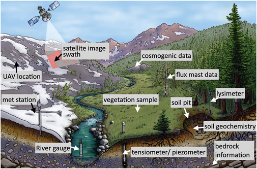
Figure 1. The Critical zone (CZ) in a mountain domain (
Banwart et al. (2011) have emphasised the significance of the CZ with reference to soils and weathering in a geochemical context:
Through unsustainable land use practices, mining, deforestation, urbanisation, and degradation by industrial pollution, soil losses are now hypothesised to be much faster (100 times or more) than soil formation (Brantley et al., 2007).
Such that:
We contend that the CZO approach is an essential advance in geoscience research and that the anticipated step change is urgently required. This is precisely because of the human pressure on the near-term habitability of Earth’s critical zone and the immense rate of ongoing environmental change. Banwart et al. (2011 p. 986).
Without extending these arguments for the CZ and for earth sciences to become more outward going and inclusive, I suggest that curricula changes (Whalley, 2022a) would be a useful way of communicating with social scientists and policymakers via publicly funded data (Boulton et al., 2012; Boulton, 2018).
Returning to the CZ, Brantley et al. (2007) indicate that,
Conceptualising the complex interplay of chemistry, biology, geology, and physics within the skin of the Earth as a system—the Critical Zone—forces scientists to work together across disciplines and scales. In so doing, scientists will learn how to interpret recurrent patterns observed in the CZ and how to protect the CZ for all life.
I now examine ways to share data and provide geo-located metadata.
Georeferencing and Sharing Data
The first two sentences of Gore’s speech about Digital Earth are:
A new wave of technological innovation is allowing us to capture, store, process, and display an unprecedented amount of information about our planet and a wide variety of environmental and cultural phenomena. Much of this information will be “georeferenced”—that is, it will refer to some specific place on the Earth’s surface.
However, it is in georeferencing that the earth sciences in general have not conformed to the concept of the Digital Earth. The Manual of Digital Earth (Guo et al., 2020), although concerned with updating Gore’s concept, does not in itself provide or recommend a geo-referencing system for datasets.
Brantley et al. (2007) illustrate the importance of locations (i.e., nodes) at the junctions of environmental gradients, suggesting localities of critical zone observatories (CZOs). In their review of CZOs, White et al. (2015) mention many monitoring “locations” of CZOs in the United States. Further, maps also include the positions of stream gauges and water samplers, soil moisture sensors, flux towers, etc., in specific watersheds and catchments. All these locations and catchments are named, sometimes with abbreviated labels. However, only one location, at Shale Hills, PA (SSHCZO) is presented more precisely than a place name (toponym): 40° 39′ 52.39″N 77° 54′ 24.23″W. However, the “precision” of this latitude/longitude is some 400 m away, northeast, from the named place on Google Earth and 400 m southeast of the named “Shaver’s Creek Environmental Centre.” In other words, although the seconds are required, this precision does not locate accurately. Another catchment mentioned with more detail in O’Geen et al. (2018) some locational data for vegetation zones but only one (37°3.120 N, 119°12.196 W) is related to a water gauging station. Thus, although the paper provides much data about this CZO, it is not easily accessible nor identifiable, even within the paper. This means that, the interoperability of the data, with other CZO locations, for example, and thus its utility, is reduced. Simple geolocation of catchments and instrumentation (Figure 1) would enhance findability, utility, and interoperability. Aspects of geochemistry in the CZ, including “hot spot” identification (Arora et al., 2022) and phosphorus and land use (Foroughi et al., 2022), would benefit from improved geolocation of sites and samples.
It is typical in most earth science case studies that data are not adequately geo-located. Other forms of geolocation have been used, especially in guidebooks and indicating field excursions. The What3Words system can have its uses and, in the United Kingdom, the British National Grid system is frequently employed. An exposure of the porphyritic andesite lava, usually known as Eycott-type after the hill of that name, is located in the English Lake District (Francis et al., 2022) at NY382296 that can be used on both paper and OS digital maps. However, it cannot be used by Google Maps or Google Earth and a search for “Eycott Hill” only gives a generalised position. A decimal 54.65899N, −2.96245W identifies this location or in dLL form, as a tuple, [54.65899, −2.96245], explained in more detail below. The decimal degree (DD) form can thus be used by anyone anywhere as it can be used in GE, OpenStreet Map, digital OS, Geology Viewer, etc., anywhere in the world. Decimal degrees, in a [dLL] format, thus provides a nodal data point that is open—findable, accessible, interoperable, and re-usable—in its own right (Whalley, 2023).
Although we may be familiar with the dms system based on the WGS84 geoid, it is not easily machine readable. It is preferable to use a decimal degree (DD) system, but this may be represented in several ways, for example, including the northings and eastings.
The [dLL] uses the square brackets to identify a decimal location that is to be treated as one value; rarely will be latitude or longitude values be useful on their own. The eastings and northings can be omitted if the convention of latitude then longitude is separated by a comma to give a comma-separated variable (CSV). A negative before a latitude gives southern hemisphere and before longitude denotes west of the prime meridian. A specification is provided elsewhere in this paper to promote acceptance of the method and methodology.
Digital Earth and Google Earth: Using [dLL] Geolocation
Grossner and Clarke (2007) examined the vision of Digital Earth in the context of the developing Google Earth (GE). Since then, GE has become an important part of visualising geoscience data (Whitmeyer et al., 2012). Having argued that good geolocation is often necessary for FAIR compliant data, I now show how it can be used by way of several earth science examples. Simply, GE can be used to supply “missing” geolocation or can be used for additional data acquisition by using the historical imagery facility.
Plate Boundary Observatory Information
Figure 2 shows an instrument site in the Salton Sea area of southern California (discovered on a bird watching trip). Its approximate location was determined by mobile phone and a subsequent search produced the basic metadata about the image given in the caption. The location on the website is given as a [dLL] pair.
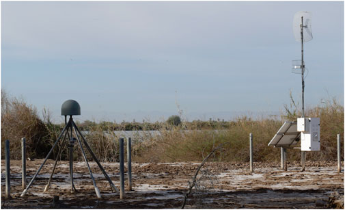
Figure 2. Earthscope Consortium Plate Boundary Observatory (PBO) GPS (GNSS) network station at Ramer Lake, near Calipatria, CA [33.0814,−115.5102]. The view direction is towards a true bearing of 205°. This is a Geodetic Facility for the Advancement of Geoscience (GAGE) with additional data at: https://www.unavco.org/data/doi/10.7283/T59P2ZKG. Image © W Brian Whalley CC BY-NC-ND 4.0.
Rock Glacier Developmental Sequence
Figure 3A shows the retrieval of a shallow ice core from below the surface debris of a rock glacier on the AGU Chapman Conference field trip to Galena Creek, WY in 1996 at [44.6444,−109.7926]. The core shows the presence of glacier ice in this rock glacier. Figure 3B shows dated Google Earth images of the same section of the rock glacier. The top horizontal line shows a reference located on the position of the core (Figure 3A) with the bottom line representing the upstream location of a small surface meltpool with its location and enlargement shown in four GE images. Imagery shows the noted locations and sizes of the meltpool in the glacier ice below the debris cover (see also Whalley, 2023). This example shows the integration of scientific literature and GE into Digital Earth.
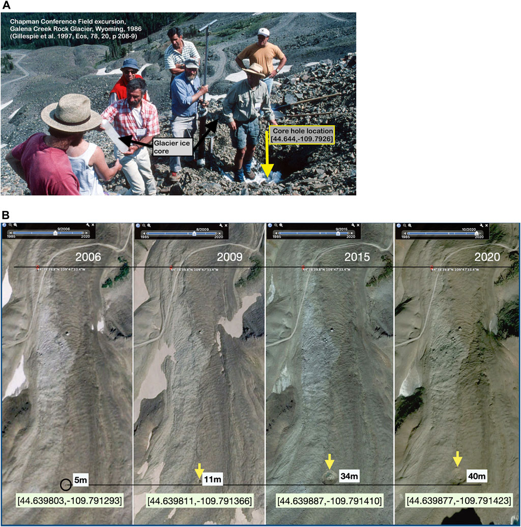
Figure 3. (A) Annotated field image recording glacier ice core retrieval from a rock glacier with the location [44.6444,−109.7926]@1996 used as a reference in (B). Noel Potter and others with corer at one of his field sites (Potter, 1972). Image ©W Brian Whalley CC BY-NC-ND 4.0. (B) A portion of Galena Creek Rock Glacier (WY, United States); local label (GCRG) with the location of a borehole showing glacier ice at [44.6444,−109.7926]. The four images show the development in size and down-valley (northward) movement of a meltpool, originally at [44.639803,−109.791293]@2006, circled and between the horizontal line and arrow points. The approximate diameter is given as measured with the GE ruler tool. Images © Google Earth and CNES/Airbus/Google Earth.
Landslide and Geomorphological Land System Mapping
A recent example of climate control on landsliding in the eastern Pamirs is given by Pei et al. (2023). No geo-located data points are provided so it is difficult to see the significance of data outliers from fitted regressions. The “overview of the landslide. sites visited” (Pei et al., 2023, Figure 6) shows the types and “triggering factors” of landslides but not their geolocations. The images used are a mix of terrestrial field site photos and Google Earth, but it is not easy to examine the landslide locations independently via GE. This is unfortunate as a paper on rock glacier mapping (Hu et al., 2023) from a similar arid area (western Kunlun Shan) indicates a debris flow planform as a “rock glacier type” used as part of a machine learning mapping project. The feature, [35.708,80.803], has been independently (Whalley et al., in preparation) assessed as a mud/debris slide and appears very similar to several examples in Pei et al. (2023). Improved geo-location and the use of GE to provide ground truth in context, rather than outlines devised for Machine Learning (ML) algorithms, would be helpful in elucidation of landforms in their climatic context. The simple expedient is to include dLL-specified geolocations, [dLL], as metadata for images, maps, and other data sources. This is much easier than reading off dms (° ‘ “) co-ordinates imprecisely from a map border. Similarly, metadata and data points in tables, lists, and inventories should be included as a matter of course. Shape and GeoTIFF files from GIS analyses alone are insufficient for FAIR data and should be supplemented by basic [dLL] located data. This should preferably be as supplementary data for a published paper with its own DOI. The AGU “Landslides Blog” (Petley, 2024) includes [dLL] identification for many events recorded as still and video images. In general, geotechnical and engineering geological mapping can be enhanced through use of [dLL] geolocation. Using a [dLL] located transect and treating the information associated with each as a “geomorphic information tensor” (Whalley, 2021) is a way to extend digital information across a wide range of geological materials using continuum mechanics (Whalley, 2024a).
Popularisation of New Findings and Geolocated Images
The magazine New Scientist recently (Dinneen, 2024) reported an explanation of gas emission craters in Siberia (Hellevang et al., 2023) and used an unidentified image (not from the cited paper) as illustration. Unfortunately, the paper itself provides no geolocated examples in the text or figures, even though it is referred to in Dinneen’s resumé. Examination by Google Earth of the approximate area in the Yamal peninsula, [68.153, 69.624], shows a wide variety of meltwater and thaw pools that are impossible to differentiate from the gas emission craters specified. Picture editors should, whenever possible, use decimal geolocations, as should authors providing “ground truth.” Another recent paper on gas emission craters (Schurmeier et al., 2024) provides additional ideas and simulations about permafrost degradation and a satellite (WorldView-1) before and after image. However, there is no georeferencing such that satellite comparisons and feature classification could be enabled. Providing a [dLL] enables more accessible data and visualisation and better communication.
Data Generation and Analysis Using dLL
The above examples show simple uses of [dLL] for finding information, metadata provision, and data analysis using Google Earth. In particular, they use a standard format to give information about a location. In effect, [dLL] are not only nodes in an information system that correspond to FAIR principles; they also specify metadata about that location. Toponyms are labels and may have descriptive shorthands, such as GCRG for Galena Creek Rock Glacier. The convenience of a [dLL] is that it can be used as well as (or instead of) a local label in a GIS or other database. Thus, a GIS is a convenient and traditional way of holding geolocated data and the development of Digital Earth has largely come from the GIS community.
Data availability of DD (decimal Latitude and longitude, as opposed to dms) may occur in some papers and be integral to them. This is all to the good when there are many factors involved from multiple papers. An example is the catalogue of “large rock-ice avalanches” produced by Schneider et al. (2011, Table 1). However, as is frequently the case, latitude and longitude are included as separate items and not as a combined value as [dLL]. How to locate such useful, but disaggregated, data in a published paper remains a problem unless its presence is already known, although retrospective references to such papers might include re-formatted data.
A Mars-dLL is already used to show the path of Mars Rovers (NASA, 2023). Not only is the path programmed, planning where the next data point will be and how the rover is to negotiate an obstacle, but the path is also shown on the website. The Rover can be seen in a Lagrangian manner, tracking back to see where it has come from. Operating on a dLL path allows tracking over time and relation to data snapshots (which may indeed be images or drill/sample points, etc.) and in probabilistic mapping (Kirkwood, this volume?). Again, a [dLL] becomes a node on a knowledge graph (Barrasa and Webber, 2023).
Making connections is traditionally done in an information context by citing an author/s as, traditionally, (adts) with a DOI now as a computer-searchable form. Figure 4 shows a simple example and Whalley (2024b) gives more complex examples. Some papers have sample data points, as, for example, the landslides by Pei et al. (2023), plotted in the paper. Souness et al. (2012) have mapped “glacier-like forms” (GLFs) on Mars. No tabular data of locations are given, and graphs are usually “averages”. Figure 5 is a simplification of one such plot (Souness et al., 2012, Figure 10) with the envelope of plotted points shown. Visualisation suggests that it is not a good statistical idea to apply linear regression as the scatter suggests confounding variables. One might ask about information concerned with the outliers and information that might be associated with their geo-locations in this use of descriptive statistics. Figure 5 shows that there may be, via visual inspection, two populations contained within the scatter. These are not commented on further here but show the possible importance of data visualisation with complex and multi-variable datasets and the use of inferential statistics on a data set.
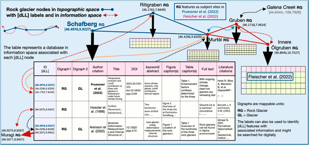
Figure 4. Basic information about a [dLL]-specified rock glacier, specifically “Schafberg RG” at [46.4976,9.9227], with the [dLL] used as a database identifier to link several references in the literature (Whalley, 2024b). Similar database tables are identified for other RG features in the European Alps, which act as nodes in a “knowledge graph.” The names of features are just convenient placeholder labels. A link is also made to the location of the GCRG [44.6444,−109.7926] which has existing author (a, d, t, s, or adts) information plus that given in Figure 2 of the present paper.
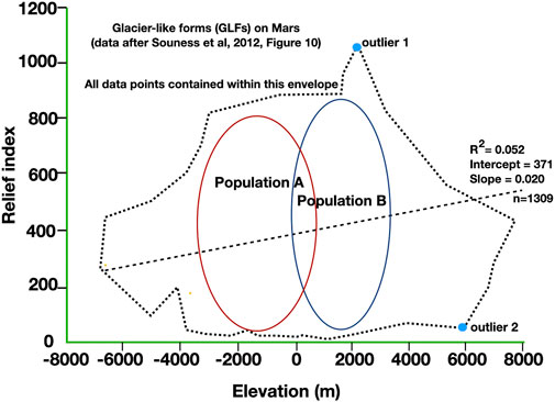
Figure 5. Bivariate representation of “glacier-like forms” (GLF) (Brough et al., 2016) on Mars after Souness et al. (2012). The “regression line” given is a rather poor fit to the data, represented here as an envelope. The characteristics of the outliers, for example, 1 and 2, might be of interest in explaining the data spread. The data in the original suggest, by eye, that there might be two merging populations of interest and evaluation, although the authors make no mention of this. Using [dLL] to identify data would be helpful in further investigations.
In astronomy, the Hertzsprung-Russell diagram plots star “luminosity” (absolute magnitude) against “colour index” (temperature for stars). Most stars, including Sol, lie on the “main sequence” while “White Dwarfs” and “Red Giants” lie below and above the main sequence with different properties. Of particular relevance here is that celestial objects can be identified, and thus instrumentation pointed at them, by their declination (=latitude) and right ascension (=longitude) in polar celestial co-ordinates. Celestial locations can then be related to information in various classification catalogues. Directing various earth science instruments at geological, geo-referenced locations would be an important way of viewing earth science and other terrestrial data. This could be illustrated by communicating Digital Earth data in CZ studies related to basin geology, relief hypsometry, etc. (Figure 1).
Data-driven models work best when there are plenty of data to use and manipulate. Remote sensing techniques, often allied with machine learning, has the capability of generating copious data points. When these are, or need to be, georeferenced then the [dLL] format is ideal as even simple spatio-temporal visualisation tools such as pivot tables and heat maps can be used to explore the data. However, Figure 5 suggests that the variance of the data hides more complex relationships than illustrated when bivariate and descriptive statistics and averages (which have statistical assumptions) are used. Without access to the data, however, there is no easy way to deconvolve the data. Where Machine Learning (ML) techniques are used to recognise images then the images themselves may need deconvolution to identify more detail and identify feature boundaries. Data augmentation techniques (Shorten et al., 2021) may also provide a way to improve data quality such that data are better fitted for purposes, whether models or for policy.
Rather than “simple”, often bivariate, data analyses (as in Figure 5), other work looking at rock glaciers from inventories (Seppi et al., 2012) show that there is a need to analyse multivariate data. Whereas rock glaciers were once studied as individual case studies (as, for example, in Figure 4), machine learning has been used to produce inventories for various purposes. A much more integrated approach is required. Using [dLL] in tables, DataFrames (as for Python), and databases is one easy way to promote this enhancement and enable better analyses.
A further advantage in using geolocation with [dLL] is the ability to use a similar system on Mars to identify and compare analogous landforms such as the “glacier-like forms” (GLF) using a Martian co-ordinate system, [dLLm]. Combined Earth-Mars data might be analysed together using visual data analysis and inferential statistics (Casella and Berger, 2024).
Pattern Recognition: Epidemics, Crime Analysis, and Geo-Heritage
With inter-correlated data, simple patterns and relationships, including spatial autocorrelation, may be hidden. The epidemiological problem of cholera solved by John Snow through his identification of the spread from the Broad Street pump in London of 1854 is well known and used as an illustration of simple graphical explanations. However, several authors have refined our knowledge of this event, for example, McLeod (2000) and, with spatial graphical analysis, Tufte (2001). Tufte (1983, p. 14) notes the title of a graph in Brier and Fienberg (1980) that deals with econometric modelling of crime and punishment, “Why one-dimensioned graphs do not always indicate influential observations.” This harks back to the data treatment mentioned in the previous section. More recently, those involved with the prevention of the spread of COVID-19 would have benefitted from the illustrative computer simulations of Grant Sanderson’s “lockdown math” as “exponential growth and epidemics” (Sanderson, 2020). Data visualisation is becoming increasingly important for analysis and communication. The recent introduction of VEDA in the NASA “EarthData” project promises to be an important platform for earth and environmental scientists in general (VEDA, 2023).
Geolocation of forensic crimes (Koch et al., 2016; Grantham et al., 2020) is an important aspect of geolocation, especially in pinpointing the scenes of crimes. This has applications directly on geo-forensics and soils forensics (Dawson, 2017; Pirrie et al., 2021), although the “predictive geolocation” of Pirrie et al. (2017) does not refer to geolocation as used in the present paper.
Landscape evolution models (LEMs) provide physically based numerical models (Temme et al., 2017), usually via digital elevation models, and provide linkages between geological, geomorphological, and hydrological parameters in a CZ context. Adding specific study information with [dLL] linkages to such models is likely to enhance their utility as predictive devices in times of rapidly changing climates. A good example in the CZ is soil erosion (Coulthard et al., 2012), where models run for tens of years under differing rainfall regimes (Hancock and Wells, 2021) assist in improving instrumentation.
In Geobritannia (Leeder and Lawlor, 2017), a popularisation of earth science to landscape, art, and literature is provided and decimal georeferencing (although not in [dLL] form) is used for many of the sites in their compilation. An example of an area of interest across earth sciences shows how [dLL] can be used and extended. Aspects of the geology and coastal engineering at a seafront promenade are described in Whalley (2022b). The refurbishment of the promenade includes several stone seats from a variety of geological sources (e.g., at [51.3515,−2.9843]) whose geological provenance might be explored in future work. Such geoheritage exploration will no doubt be helped by the use of digital technologies coupled to UAV affordability and utility (Foster, 2023) and Google Earth-based field guides.
A recent paper by Worsley (2018) examines some sites in Shropshire, United Kingdom, visited as part of Charles Darwin’s pre-Beagle geological experiences. UK National Grid referencing is used, but this can be converted to [dLL] format, and locations can also be associated with Darwin in North Wales and “Darwin’s Boulders” in Cwm Idwal (Smith, 2024) and in Patagonia, [−53.406,−68.077], (Evenson et al., 2009, Figure 5). A digital “Darwin geological trail” could be developed using [dLL] as a Google Earth tour and concentrated in a kmz file. Whitmeyer et al. (2012) provide a good introduction to how some of these aspects of digital sciences can be introduced into earth science education.
Specifying [dLL]: Their Use and Utility
To create a dLL, place decimal degrees, first latitude then longitude, inside square brackets separated by a comma. For example: [51.50864,−0.13852].
Coordinate System
The WGS84/EPSG:4326 coordinate reference system must be used.
Decimal Representation
Latitude is ±90, with positive values denoting north of the equator and negative values denoting south. Longitude is ±180, with positive values denoting east of the prime meridian and negative values denoting west.
Four or five decimal places should be sufficient for most place locations, with five places providing precision of about a metre.1
Reducing precision, fewer than 2 decimal places, in order to refer to a wide area, is discouraged.
Optional Date and Direction
If a year is needed for the correct interpretation of the location, it can be provided after the latitude and longitude, for example, [53.67543,−0.38033]@2003. A second element might be added as a direction facing the image. This is a true bearing in whole degrees with reference to north. This might be used, for example, to show the direction of a photograph, as in Figure 2; [33.0814,−115.5102], 205.
Typesetting
The negative symbol should be a hyphen-minus, ASCII 45/0x2D, Unicode U+002D, normally used as a hyphen, or in mathematical expressions, as a minus sign.
The square bracket should be ASCII 91/0x5b, Unicode U+005B; and ASCII 93/0x5d, Unicode U+005D, respectively.
The comma should be ASCII 44/0x2c, Unicode U+002C.
When viewed on a computer, as for proofing and checking, it should be possible to copy a [dLL] and paste it directly and unambiguously into, e.g., Google Maps and Google Earth. It should not be split across a line break.
Table 1 is an example of a data table, for instance in supplementary material for a paper or the initial stages of a data repository with [dLL] referencing.
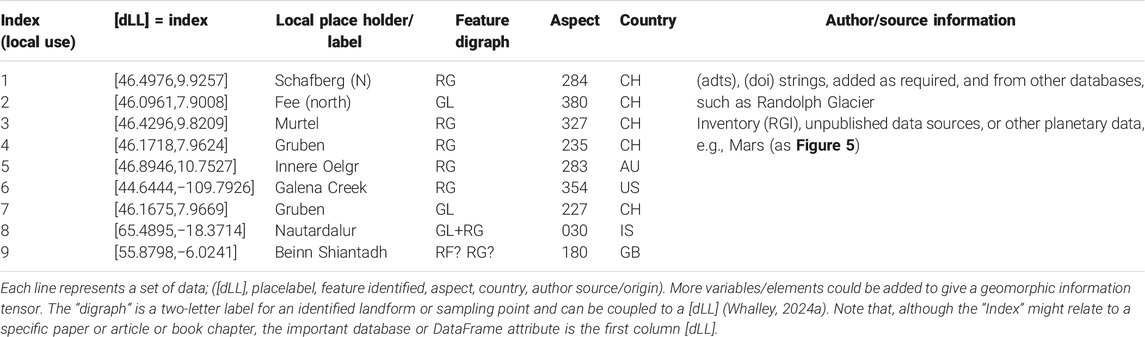
Table 1. A simple [dLL]-specified set of entries for a feature inventory using Figure 4 as a basis.
In Table 1, note that [dLL], including the square brackets, can be pasted into other open data sources. For example, the Swiss examples can be inserted into the SwissTopo “Journey through time” map’s search bar (Whalley, 2020) and the British Geological Survey (BGS) “Geology Viewer” can also be used with the “full” [dLL] expression to provide geological information as well as the Ordnance Survey mobile digital maps. These abilities show the utility of the [dLL] format. Table 1 refers to identification of features and their geolocation. This maximises the usefulness of the data via the FAIR principles. Geolocated data used in a publication should be made available to exploit further, for example, in another dataset at another time, as in Figure 3B. In econometrics, panel data (pandas) are data sets that include observations over multiple time periods. Geolocated data should be available as simple CSV strings using [dLL] as headers for each entry (see the comments of Berners-Lee in Open and FAIR Data section). Such data files should be the prime form of record with shape or KMZ files only as additions.
Analytical data should be presented, especially in table format, with a [dLL] row header where the data need to be geo-located. Accessibility and re-usability are important, not least because laboratory analyses are expensive. Cosmogenic ratio data, for example, frequently have laboratory codes as the row identifier or a local name label but without proper geolocation. Increasingly latitude longitude data are given but as two separate entries. Placing them together in a [dLL] would achieve their inclusion and enhance their utility under the FAIR principles.
Discussion and Implications
The need for digital data is predicated on data models that require organised data. Good geolocation assists this objective and can be optimised by relating one to another, as in Digital Earth. Data structures can be used to test ideas derived from, usually deterministic, models but also to explore inductive and probabilistic approaches to data analysis. In his discussion on “building confidence in geological models,” Bowden (2004) noted that, “In general terms, models are required because we do not have complete knowledge, in time or in space, of the system of interest.” Bowden’s chapter repays attention as we move into an era of more digital data and with the warning, “Where is the information we have lost in data?” (Inose and Pierce, 1984).
Collections of data, such as those used by some ML devices in remote sensing, collect data and use inductive data processing to see “what might be there.” In simple terms, results like Figure 5 might result from descriptive statistics. However, if data points can be identified by geolocation then a variety of visualisation techniques can be used to interpret the set better and to allow comparisons between data sets. Visualisation of complex data should now be possible with relatively inexpensive headsets. Such techniques may be at least as informative as a virtual field class walking virtually (augmented reality—AR or virtual reality—VR) on the ground (Cleverley, this volume) or inspecting a section or examining a borehole log or seismic trace (Dommisse et al., this volume). A point cloud of (Lidar-produced) data could also have an associated metadata cloud that could be used for future data gathering and interpretation. Google Earth Engine is a cloud-based “planetary-scale platform for Earth science data and analysis” containing satellite and geospatial datasets that have much potential for earth and environmental scientists to produce big digital data sets (Chen et al., 2020). Useful reviews and meta-analyses have recently been provided by Tamiminia et al. (2020) and Yang et al. (2022).
The construction of knowledge graphs suggests ways in which nodes, or vertices, (such as [dLL]) are connected entities and where the connections (edges) are relationships. Figure 4 shows how a tree structure might be formed as more [dLL] connections are added (Table 1). The simple, and traditional, toponym labels are supplemented by [dLL] and knowledge graphs could be constructed for further analysis. In a CZ context, a location or sample site has information about the solid geology, added to which could be information about the surface materials, soil properties, agricultural potential, runoff characteristics, and so on (Figure 1). Such an information structure also helps in making suggestions about where sampling should be done.
A further possibility, especially related to specialised features such as “landslide rock glacier” is to use a Wiki structure as a way of organising data (Mehler, 2008). In any event, RDF triple structures (schemas) are likely to provide an initial way of structuring data to use in ontologies and classification schemes. An RDF schema, as a Worldwide Web Consortium, W3C, was first proposed to help organise metadata as a data model and is also a means of describing and exchanging data. This gives the subject (as a node) connected to a node for the object being connected by a link, the predicate. A collection of RDF triples can be used to produce a directed (multi)graph. Semantic Wikis (Schaffert et al., 2008) may be a good way of exploring the structure building of the Semantic Web and knowledge trees with ease of use and data input. This sort of structure would be better than an inventory (often with opaque or non-open data). For example, the landslide examples of Pei et al. (2023) could be built into a wiki with “type forms” identified and, if necessary, queried and supplemented for future investigations. The use of [dLL] would be fundamental to such advanced data modelling. As with animal tracking, especially birds, kinematics with small GPS loggers are increasingly effective in increasing linear/spatial data. When added to satellite/UAV-derived data using techniques such as “structure from motion” and InSAR, geo-located data are amplified greatly. Data analysis techniques, especially those related to knowledge graphs and Large Language Models (LLMs), are now available with commercial and open-source versions.
Such benefits also accrue by associating information at instrumented CZO catchments, as mentioned previously, and in the increasing use of Digital Twins (National Academy of Science Engineering and Medicine, 2023). The types of uncertainty discussed by Bowden (2004) and the emergence of complex systems (Funtowicz and Ravetz, 1994) realised by increasing amounts of digital data can raise public policy and decision-making issues regarding data quality in “post-normal science” (Karpińska, 2018). Using more open data and science as an “open enterprise” (Boulton et al., 2011; Boulton et al., 2012) will be helpful in the earth sciences and beyond.
The use of [dLL] is established as a basic means of providing FAIR-compliant geolocation. Tools are being developed to show how [dLL] can be used in a variety of ways. However, we can recommend that [dLL] be used as a matter of course to provide and locate metadata for earth science resources, especially as used in papers and reports. For example, appropriate [dLL] could be added to “Keywords” lists or in the title. In a paper it is usual to cite “previous work,” but it would be helpful for a list of georeferenced locations to be included as a distinct, searchable, entity of a paper, see Whalley (2022c, 2024b). Local labels alone, for example, as in Figure 4, should be supplemented by [dLL] specifications (“Which Darwin Boulders do you mean?”). Further, the basic data used to compile data for a table, graph, or inventory should be available as a supplement to the paper with its own DOI and not left for the potential user to “contact the author.” Some issues related to FAIR data curation are presented by Giannini and Molino (2018) and implementation by Jacobsen et al. (2020).
There are implications for earth science education in the findings and suggestions in this paper, where using AI and LLM are a part of geolocated data analysis within the Digital Earth concept. Training in data analysis should become more central to ‘thinking like a geologist’ via investigating the complexities of the “Bretherton Diagram” (Manduca and Kastens, 2012), which includes aspects of the Critical Zone in relationships to other disciplines. Further, there is no reason why data analysts should not become earth science data analysts and help address some cultural biases. As Shafer et al. (2024, p 8) suggest, “Efforts to ensure that geoscience fields are welcoming and accessible to people with physical disabilities must address barriers to entry in geoscience careers, as well as the development of a more inclusive and culturally responsive workplace.”
Conclusion
The Digital Earth data model provides a ubiquitous way to collect and envision data for the benefit of all. Using information associated with Digital Earths in a wise manner, as recommended by Boulton et al. (2011), is significant. Not the least of the requirements is the FAIR sharing of data and the ability to update and upgrade our knowledge of the world. Structuring data is as important as its generation, storage and processing, and dissemination. The widespread use of [dLL] geolocation is a significant step towards better use of Digital Earth.
A [dLL] is a simple enabling device that enhances data utility. They are easy to insert into metadata and written material, which then provides a generally accessible and FAIR-compliant georeferencing system. Such a system has, so far, been mostly absent from geoscience contributions to the Digital Earth. Associating [dLL] with site information allows extension of basic GIS systems and cross-linking data and information. Case-based observations and systematically collected data can be made more open and thus increase the usage of earth science data as our ability to visualise and model earth data.
Author Contributions
The author confirms being the sole contributor of this work and has approved it for publication.
Funding
The author declares that no financial support was received for the research, authorship, and/or publication of this article.
Conflict of Interest
The author declares that the research was conducted in the absence of any commercial or financial relationships that could be construed as a potential conflict of interest.
Publisher’s Note
All claims expressed in this article are solely those of the authors and do not necessarily represent those of their affiliated organizations, or those of the publisher, the editors and the reviewers. Any product that may be evaluated in this article, or claim that may be made by its manufacturer, is not guaranteed or endorsed by the publisher.
Acknowledgments
I thank Andrew R. Whalley for discussion and insights and Google Earth for use of the credited images. This paper is dedicated to the late Prof. Steve Banwart (1959–2023), Founder of the Global Food and Environment Institute, University of Leeds.
Footnotes
1https://en.wikipedia.org/wiki/Decimal_degrees#Precision
References
Arora, B., Briggs, M. A., Zarnetske, J. P., Stegen, J., Gomez-Velez, J. D., Dwivedi, D., et al. (2022). “Hot Spots and Hot Moments in the Critical Zone: Identification of and Incorporation Into Reactive Transport Models,” in Biogeochemistry of the Critical Zone. Editors A. S. Wymore, W. H. Yang, W. L. Silver, W. H. McDowell, and J. Chorover (Springer), 9–47. doi:10.1007/1978-1003-1030-95921-95920_95922
Banwart, S., Bernasconi, S. M., Bloem, J., Blum, W., Brandao, M., Brantley, S., et al. (2011). Soil Processes and Functions in Critical Zone Observatories: Hypotheses and Experimental Design. Vadose Zone J. 10 (3), 974–987. doi:10.2136/vzj2010.0136
Barrasa, J., and Webber, J. (2023). Building Knowledge Graphs. A Practitioner’s Guide. Sebastopol, CA: O’Reilly.
Berners-Lee, T. (2010). Is Your Linked Open Data 5 Star? Available at: https://www.w3.org/DesignIssues/LinkedData.html.
Berners-Lee, T., Hendler, J., and Lassila, O. (2001). The Semantic Web. Sci. Am. 284 (5), 34–43. doi:10.1038/scientificamerican0501-34
Boulton, G. (2018). The Challenges of a Big Data Earth. Big Earth Data 2 (1), 1–7. doi:10.1080/20964471.2017.1397411
Boulton, G., Campbell, P., Collins, B., Elias, P., Hall, W., Laurie, G., et al. (2012). Science as an Open Enterprise. Open Communication of Data: The Source of a Scientific Revolution and of Scientific Progress. The Royal Society, Report. Available at: https://www.royalsociety.org.
Boulton, G., Rawlins, M., Vallance, P., and Walport, M. (2011). Science as a Public Enterprise: The Case for Open Data. Lancet 377 (9778), 1633–1635. doi:10.1016/s0140-6736(11)60647-8
Bowden, R. A. (2004). “Building Confidence in Geological Models,” in Geological Prior Information. Editors A. Curtis, and R. Wood (London: Geological Society, London, Special Publication), 157–173. doi:10.1144/GSL.SP.2004.239.01.11
Brantley, S. L., Goldhaber, M. B., and Ragnarsdottir, K. V. (2007). Crossing Disciplines and Scales to Understand the Critical Zone. Elements 3 (5), 307–314. doi:10.2113/gselements.3.5.307
Brier, S. S., and Fienberg, S. E. (1980). Recent Econometric Modeling of Crime and Punishment: Support for the Deterrence Hypothesis? Eval. Rev. 4 (2), 147–191. doi:10.1177/0193841x8000400201
Brough, S., Hubbard, B., and Hubbard, A. (2016). Former Extent of Glacier-Like Forms on Mars. Icarus 274, 37–49. doi:10.1016/j.icarus.2016.03.006
Chen, L., Wang, L., Miao, J., Gao, H., Zhang, Y., Yao, Y., et al. (2020). Review of the Application of Big Data and Artificial Intelligence in Geology. J. Phys. Conf. Ser. 1684, 012007. doi:10.1088/1742-6596/1684/1/012007
Coulthard, T. J., Hancock, G. R., and Lowry, J. B. (2012). Modelling Soil Erosion With a Downscaled Landscape Evolution Model. Earth Surf. Process. Landforms 37 (10), 1046–1055. doi:10.1002/esp.3226
Crüwell, S., Van Doorn, J., Etz, A., Makel, M. C., Moshontz, H., Niebaum, J. C., et al. (2019). Seven Easy Steps to Open Science. Z. für Psychol. 227 (4), 237–248. doi:10.1027/2151-2604/a000387
Dawson, L. (2017). Soil Organic Characterisation in Forensic Case Work. Episodes J. Int. Geoscience 40 (2), 157–165. doi:10.18814/epiiugs/2017/v40i2/017018
Dinneen, J. (2024). Siberia’s Mysterious Craters May Have Been Carved Out by Hot Gas Explosions. New Sci. 261 (3474), 9. doi:10.1016/s0262-4079(24)00097-6
Dublin Core (2005). Using Dublin Core. Available at: https://www.dublincore.org/specifications/dublin-core/usageguide/.
Evenson, E. B., Burkhart, P. A., Gosse, J. C., Baker, G. S., Jackofsky, D., Meglioli, A., et al. (2009). Enigmatic Boulder Trains, Supraglacial Rock Avalanches, and the Origin of" Darwin's Boulders," Tierra del Fuego. GSA Today 19 (12), 4–10. doi:10.1130/gsatg72a.1
Foroughi, M., Sutter, L. A., Richter, D., and Markewitz, D. (2022). “Hillslope Position and Land-Use History Influence P Distribution in the Critical Zone,” in Biogeochemistry of the Critical Zone. Editors A. S. Wymore, W. H. Yang, W. L. Silver, W. H. McDowell, and J. Chorover (Springer), 171–202. doi:10.1007/978-3-030-95921-0
Francis, I., Holmes, S., and Yardley, B. (2022). The Lake District, Landscape and Geology. Marlborough: Crowood Press.
Funtowicz, S., and Ravetz, J. R. (1994). Emergent Complex Systems. Futures 26 (6), 568–582. doi:10.1016/0016-3287(94)90029-9
Giannini, S., and Molino, A. (2018). “The Data Librarian: Myth, Reality or Utopia,” in GL20 Proceeding: Twentieth International Conference on Grey Literature “Research Data Fuels and Sustains Grey Literature, New Orleans, USA, December 3-4, 2018.
Gore, A. (1999). The Digital Earth: Understanding Our Planet in the 21st Century. Aust. Surv. 43, 89–91. doi:10.1080/00050326.1998.10441850
Grantham, N. S., Reich, B. J., Laber, E. B., Pacifici, K., Dunn, R. R., Fierer, N., et al. (2020). Global Forensic Geolocation With Deep Neural Networks. J. R. Stat. Soc. Ser. C Appl. Statistics 69 (4), 909–929. doi:10.1111/rssc.12427
Grossner, K., and Clarke, K. (2007). “Is Google Earth,“Digital Earth?”: Defining a Vision,” in Proceedings of the Fifth International Symposium on Digital Earth (University Park, PA: CiteSeer).
H. Guo, M. F. Goodchild, and A. Annoni (2020). Manual of Digital Earth (Springer Open). doi:10.1007/978-981-32-9915-3
Hancock, G., and Wells, T. (2021). Predicting Soil Organic Carbon Movement and Concentration Using a Soil Erosion and Landscape Evolution Model. Geoderma 382, 114759. doi:10.1016/j.geoderma.2020.114759
Hasnain, A., and Rebholz-Schuhmann, D. (2018). “Assessing FAIR Data Principles Against the 5-Star Open Data Principles,” in The Semantic Web: ESWC 2018 Satellite Events: ESWC 2018 Satellite Events, Heraklion, Crete, Greece, June 3-7, 2018, Revised Selected Papers 15. Lecture Notes in Computer Science (Springer). doi:10.1007/978-3-319-98192-5
Hellevang, H., Ippach, M. R., Westermann, S., and Nooraiepour, M. (2023). Formation of Giant Siberian Gas Emission Craters (GECs). EarthArXiv. doi:10.31223/x59q3k
Hu, Y., Liu, L., Huang, L., Zhao, L., Wu, T., Wang, X., et al. (2023). Mapping and Characterizing Rock Glaciers in the Arid Western Kunlun Mountains Supported by InSAR and Deep Learning. J. Geophys. Res. Earth Sci. 128. doi:10.1029/2023JF007206
Inose, H., and Pierce, J. R. (1984). Information Technology and Civilization. World Futur. J. General Evol. 19 (3-4), 293–303. doi:10.1080/02604027.1984.9971988
Jacobsen, A., De Miranda Azevedo, R., Juty, N., Batista, D., Coles, S., Cornet, R., et al. (2020). FAIR Principles: Interpretations and Implementation Considerations. Data Intell. 2, 10–29. doi:10.1162/dint_r_00024
Karpińska, A. (2018). Post-Normal Science. The Escape of Science: From Truth to Quality? Soc. Epistemol. 32 (5), 338–350. doi:10.1080/02691728.2018.1531157
Koch, R., Golling, M., Stiemert, L., and Rodosek, G. D. (2016). Using Geolocation for the Strategic Preincident Preparation of an It Forensics Analysis. IEEE Syst. J. 10 (4), 1338–1349. doi:10.1109/jsyst.2015.2389518
Leeder, M., and Lawlor, J. (2017). GeoBritannica. Edinburgh and London: Dunedin academic press limited.
Manduca, C. A., and Kastens, K. A. (2012). “Mapping the Domain of Complex Earth Systems in the Geosciences,” in Earth and Mind II: A Synthesis of Research on Thinking and Learning in the Geosciences. Editors K. A. Kastens, and C. A. Manduca (American Geological Society), 91–96. Special Paper 486. doi:10.1130/2012.2486(16)
Mcleod, K. S. (2000). Our Sense of Snow: The Myth of John Snow in Medical Geography. Soc. Sci. Med. 50 (7-8), 923–935. doi:10.1016/s0277-9536(99)00345-7
Mehler, A. (2008). Structural Similarities of Complex Networks: A Computational Model by Example of Wiki Graphs. Appl. Artif. Intell. 22 (7-8), 619–683. doi:10.1080/08839510802164085
NASA (2023). Where Is Perseverance? Available at: https://mars.nasa.gov/mars2020/mission/where-is-the-rover/.
National Academy of Science Engineering and Medicine (2023). Foundational Research Gaps and Future Directions for Digital Twins. Washington DC: National Academies Press. doi:10.17226/26894
O'Geen, A., Safeeq, M., Wagenbrenner, J., Stacy, E., Hartsough, P., Devine, S., et al. (2018). Southern Sierra Critical Zone Observatory and Kings River Experimental Watersheds: A Synthesis of Measurements, New Insights, and Future Directions. Vadose Zone J. 17 (1), 1–18. doi:10.2136/vzj2018.04.0081
Pei, Y., Qiu, H., Zhu, Y., Wang, J., Yang, D., Tang, B., et al. (2023). Elevation Dependence of Landslide Activity Induced by Climate Change in the Eastern Pamirs. Landslides 20, 1115–1133. doi:10.1007/s10346-023-02030-w
Petley, D. (2024). The Landslide Blog. Available at: https://blogs.agu.org/landslideblog/ (Accessed March 30, 2024).
Pirrie, D., Dawson, L., and Graham, G. (2017). Predictive Geolocation: Forensic Soil Analysis for Provenance Determination. Episodes J. Int. Geoscience 40 (2), 141–147. doi:10.18814/epiiugs/2017/v40i2/017016
Pirrie, D., Ruffell, A., Dawson, L., and Mckinley, J. (2021). “Crime Scenes: Geoforensic Assessment, Sampling and Examination,” in A Guide to Forensic Geology. Editors L. J. Donnelly, D. Pirrie, M. Harrison, A. Ruffell, and L. Dawson (London: Geological Society of London), 87–110.
Potter, N. (1972). Ice-Cored Rock Glacier, Galena Creek, Northern Absaroka Mountains, Wyoming. Geol. Soc. Am. Bull. 83 (10), 3025–3058. doi:10.1130/0016-7606(1972)83[3025:IRGGCN]2.0.CO;2
Rasmussen, C., Troch, P. A., Chorover, J., Brooks, P., Pelletier, J., and Huxman, T. E. (2011). An Open System Framework for Integrating Critical Zone Structure and Function. Biogeochemistry 102 (1-3), 15–29. doi:10.1007/s10533-010-9476-8
Sanderson, G. (2020). Lockdown Math. Exponential Growth and Epidemics 3blue1Brown. Available at: https://www.youtube.com/watch?v=Kas0tIxDvrg&t=326s.
Schaffert, S., Bry, F., Baumeister, J., and Kiesel, M. (2008). Semantic Wikis. IEEE Softw. 25 (4), 8–11. doi:10.1109/ms.2008.95
Schneider, D., Huggel, C., Haeberli, W., and Kaitna, R. (2011). Unraveling Driving Factors for Large Rock–Ice Avalanche Mobility. Earth Surf. Process. Landforms 36 (14), 1948–1966. doi:10.1002/esp.2218
Schurmeier, L. R., Brouwer, G. E., and Fagents, S. A. (2024). Formation of the Siberian Yamal Gas Emission Crater via Accumulation and Explosive Release of Gas Within Permafrost. Permafr. Periglac. Process. 35 (1), 33–45. doi:10.1002/ppp.2211
Seppi, R., Carton, A., Zumiani, M., Dall'amico, M., Zampedri, G., and Rigon, R. (2012). Inventory, Distribution and Topographic Features of Rock Glaciers in the Southern Region of the Eastern Italian Alps (Trentino). Geogr. Fis. Din. Quaternaria 35, 185–197. doi:10.4461/GFDQ.2012.35.17
Shafer, G., Viskupic, K., and Egger, A. (2024). Geoscience Job Advertisements as a Barrier to Employment for People With Disabilities. Earth Sci. Syst. Soc. 4, 10086. doi:10.3389/esss.2024.10086
Shorten, C., Khoshgoftaar, T. M., and Furht, B. (2021). Text Data Augmentation for Deep Learning. J. Big Data 8, 101–134. doi:10.1186/s40537-021-00492-0
Smith, N. (2024). Cwm Idwal and Darwin’s Boulders. Available at: https://www.geolsoc.org.uk/GeositesCwmIdwal.
Souness, C., Hubbard, B., Milliken, R. E., and Quincey, D. (2012). An Inventory and Population-Scale Analysis of Martian Glacier-Like Forms. Icarus 217 (1), 243–255. doi:10.1016/j.icarus.2011.10.020
Tamiminia, H., Salehi, B., Mahdianpari, M., Quackenbush, L., Adeli, S., and Brisco, B. (2020). Google Earth Engine for Geo-Big Data Applications: A Meta-Analysis and Systematic Review. ISPRS J. Photogrammetry Remote Sens. 164, 152–170. doi:10.1016/j.isprsjprs.2020.04.001
Temme, A., Armitage, J., Attal, M., Van Gorp, W., Coulthard, T., and Schoorl, J. (2017). Developing, Choosing and Using Landscape Evolution Models to Inform Field-Based Landscape Reconstruction Studies. Earth Surf. Process. Landforms 42 (13), 2167–2183. doi:10.1002/esp.4162
Tufte, E. R. (1983). The Visual Display of Quantitative Information. Cheshire, Conn: Graphics Press.
Tufte, E. R. (2001). Visual Explanations: Images and Quantities, Evidence and Narrative. Cheshire, Conn: Graphics Press.
VEDA (2023). Introducing VEDA: An Open Science Platform to Accelerate Earth Science Research and Application. Available at: https://www.earthdata.nasa.gov/learn/blog/veda-open-science-platform.
Waldron, P. (2020). Critical Zone Science Comes of Age. Eos Trans. Am. Geophys. Union 101 (24). doi:10.1029/2020EO148734
Whalley, W. B. (2020). Gruben Glacier and Rock Glacier, Wallis, Switzerland: Glacier Ice Exposures and Their Interpretation. Geogr. Ann. Ser. A, Phys. Geogr. 102 (2), 141–161. doi:10.1080/04353676.2020.1765578
Whalley, W. B. (2021). Mapping Small Glaciers, Rock Glaciers and Related Features in an Age of Retreating Glaciers: Using Decimal Latitude-Longitude Locations and 'Geomorphic Information Tensors. Geogr. Fis. Din. Quaternaria 44, 55–67. doi:10.4461/GFDQ.2021.44.4
Whalley, W. B. (2022a). On Teaching Geomorphology: Making It More Scientific via the Critical Zone Concept. Geography 107 (2), 85–96. doi:10.1080/00167487.2022.2068840
Whalley, W. B. (2022b). Earth Science, Art and Coastal Engineering at the Seaside: Envisioning an Open Exploratorium or Geo-Promenade at Weston-Super-Mare, Somerset, United Kingdom. Geoheritage 14, 113. doi:10.1007/s12371-022-00745-1
Whalley, W. B. (2022c). Figures, Landscapes and Landsystems: Digital Locations, Connectivity and Communications. Earth Surf. Process. Landforms 47, 2173–2177. doi:10.1002/ESP.5418
Whalley, W. B. (2023). Landscape Domains and Information Surfaces: Data Collection, Recording and Citation Using Decimal Latitude-Longitude Geolocation via the FAIR Principles. Earth Surf. Process. Landforms 48, 2141–2151. doi:10.1002/esp.5678
Whalley, W. B. (2024a). Glacier–Rock Glacier Interactions in the Eastern Hindu Kush, Nuristan, Afghanistan [35.92,71.13] in the Period 1976-2019. Geogr. Ann. Ser. A Phys. Geogr. 105, 1–30. doi:10.1080/04353676.2024.2321425
Whalley, W. B. (2024b). The Geolocation of Features on Information Surfaces and the Use of the Open and FAIR Data Principles in the Mountain Landscape Domain and Geoheritage. Permafr. Periglac. Process. 35, 98–108. doi:10.1002/ppp.2217
White, T., Brantley, S., Banwart, S., Chorover, J., Dietrich, W., Derry, L., et al. (2015). “The Role of Critical Zone Observatories in Critical Zone Science,” in Developments in Earth Surface Processes (Elsevier), 15–78. doi:10.1016/b1978-1010-1444-63369-63369.00002-63361
S. J. Whitmeyer, J. E. Bailey, D. G. De Paor, and T. Ornduff (2012). Google Earth and Virtual Visualizations in Geoscience Education and Research (Boulder: Geological Society of America). Special Paper 492. doi:10.1130/2012.2492(00)
Wilkinson, M. D., Dumontier, M., Aalbersberg, I. J., Appleton, G., Axton, M., Baak, A., et al. (2016). The FAIR Guiding Principles for Scientific Data Management and Stewardship. Sci. Data 3 (1), 160018–160019. doi:10.1038/sdata.2016.18
Wilkinson, M. D., Dumontier, M., Jan Aalbersberg, I., Appleton, G., Axton, M., Baak, A., et al. (2019). Addendum: The FAIR Guiding Principles for Scientific Data Management and Stewardship. Sci. Data 6 (1), 6. doi:10.1038/s41597-019-0009-6
Worsley, P. (2018). Charles Darwin’s 1831 Geological Fieldwork in Shropshire. Mercian Geol. 19 (3), 160–168.
Keywords: Digital Earth, critical zone science, [dLL], geolocation, georeferencing, visualisation, modelling
Citation: Whalley WB (2024) Enhancing the Digital Earth via Digital Decimal Geolocation and the FAIR Data Principles. Earth Sci. Syst. Soc. 4:10110. doi: 10.3389/esss.2024.10110
Received: 24 January 2024; Accepted: 12 April 2024;
Published: 02 May 2024.
Edited by:
Jennifer M. McKinley, Queen’s University Belfast, United KingdomReviewed by:
Tom Coulthard, University of Hull, United KingdomAlastair Ruffell, Queen’s University Belfast, United Kingdom
Copyright © 2024 Whalley. This is an open-access article distributed under the terms of the Creative Commons Attribution License (CC BY). The use, distribution or reproduction in other forums is permitted, provided the original author(s) and the copyright owner(s) are credited and that the original publication in this journal is cited, in accordance with accepted academic practice. No use, distribution or reproduction is permitted which does not comply with these terms.
*Correspondence: W. Brian Whalley, b.whalley@sheffield.ac.uk